Advanced Formatting Techniques for Creating AER Quality Plots

by aptech · Published July 27, 2022 · Updated July 28, 2022

Introduction

Today's blog will show you how to reproduce one of the graphs from a paper in the June 2022 issue of the journal, American Economic Review. You will learn how to:

1. Add and style text boxes with LaTeX.
2. Set the anchor point of text boxes.
3. Add and style vertical lines.
4. Automatically set legend text to use your dataframe's variable names.
5. Set the font for all or a subset of the graph text elements.
6. Set the size of your graph.

The Graph and Data

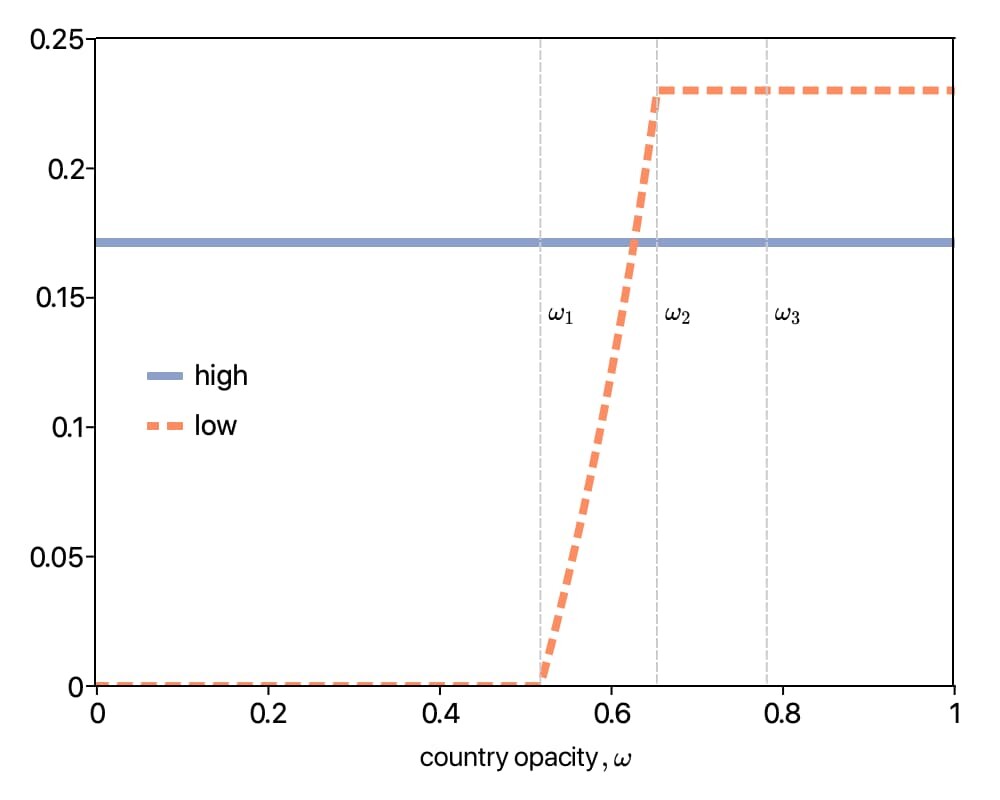
Below is the graph that we are going to create. It is adapted from a recent paper in the American Economic Review. You can download the data here.

Load and Preview Data

Our first step will be to load the data and take a quick look at it.

// Load all variables from 'int_rate.csv'
int_rate = loadd("int_rate.csv");

// Print the first 5 observations of 'int_rate'
print "First 5 observations:";
head(int_rate);

// Print the last 5 observations of 'int_rate'
print "Last 5 observations:";
tail(int_rate);

// Print descriptive statistics of our variables
call dstatmt(int_rate);

This will give us the following results:

First 5 observations:

               x             high              low
   0.00010000000       0.17140598        0.0000000
   0.00020000000       0.17140598        0.0000000
   0.00030000000       0.17140598        0.0000000
   0.00040000000       0.17140598        0.0000000
   0.00050000000       0.17140598        0.0000000

Last 5 observations:

               x             high              low
      0.99950000       0.17140598       0.23012203
      0.99960000       0.17140598       0.23012203
      0.99970000       0.17140598       0.23012203
      0.99980000       0.17140598       0.23012203
      0.99990000       0.17140598       0.23012203

-------------------------------------------------------------------------------
Variable     Mean    Std Dev     Variance    Minimum    Maximum   Valid Missing
-------------------------------------------------------------------------------

x             0.5      0.289       0.0833      1e-4      0.999    9999    0
high       0.1714   1.04e-07     1.08e-14     0.171      0.171    9999    0
low       0.09374      0.108       0.0116         0      0.230    9999    0

Initial Graphs

Our first graphs will use the default GAUSS styling. We will create one graph indexing our x and y variables and another using a formula string.

Indexing

// Set our graph size to 500x400 pixels
plotCanvasSize("px", 500 | 400);

// Use indexing to select the 'x' and 'y' variables
plotXY(int_rate[.,"x"], int_rate[.,"high" "low"]);

Formula string

// Set our graph size to 500x400 pixels
plotCanvasSize("px", 500 | 400);

// Specify the 'x' and 'y' variables using a formula string
plotXY(int_rate, "high + low ~ x");

When we use a formula string with our plot functions, it tells GAUSS that we want to use the information from the dataframe.

When using a formula string in plots:

• The tilde symbol, ~, separates the y variables on the left from the x variable(s) on the right.
• If there is a single y variable, GAUSS will use that variable name to label the y axis. If there is more than one y variable, then the variable names will be added to the legend.
• The name of the x variable will be used to label the x-axis.

While this may not always be the information we want to be displayed in our final plot, it makes it convenient to quickly create graphs that are easier to interpret.

Plot Styling

Fp Next, we will adjust the styling to match our intended final plot.

To programmatically style our graph, the first thing we need to do is to create a plotControl structure and fill it with default values.

struct plotControl plt;
plt = plotGetDefault("xy");

Legend styling

After the pointer to the plotControl structure we want to modify, &plt, the function plotSetLegend takes one required input and two optional ones.

1. Legend text: This controls the text that will be displayed in the legend. We want GAUSS to use the variable names from our input. Therefore, below, we set this to an empty string, "". This tells GAUSS that we do not want to modify the default behavior of the legend text.

   As we mentioned earlier, the default behavior for a graph created with a formula string with more than one y variable is to use the y variable names as the legend text elements.

2. Legend location: This input can be a string with text location specifications, or a 2x1 vector with the x and y coordinates for the location of the top-left corner of the legend.

3. Legend orientation: This input specifies whether the legend position should be stacked vertically or horizontally. We set it to 1 to indicate a vertical arrangement. It may help to remember that a 1 is a vertical essentially a vertical mark.

The first input to plotSetLegendBkd, after the plotControl structure pointer, controls the legend opacity. We set it to be 0% opaque, or 100% transparent.

plotSetLegend(&plt, "", "vcenter left inside", 1);
plotSetLegendBkd(&plt, 0);

Font styling

plotSetFonts provides a convenient way to set the font family, size, and color for any subset of the text in your graph. Below we set the font for 'all' of the text in the plot. However, there are many other options, including: "axes", "legend", "legend_title", "title", "ticks" and many more.

plotSetFonts(&plt, "all", "roboto", 14);

X-axis label

plotSetTextInterpreter tells GAUSS whether you would like text labels to be interpreted as:

• HTML
• LaTeX
• Plain text

Like plotSetFonts, it allows you to specify many different locations, or even, "all". Below, we set the x-axis to be interpreted as LaTeX and then use LaTeX in our x-axis label.

plotSetTextInterpreter(&plt, "latex", "xaxis");
plotSetXAxisLabel(&plt, "\\text{country opacity }, \\omega");

Main line styling

The "set2" color palette contains eight colors:

We want to use the third color for our first series, "high", and the second color for our second series, "low".

Additionally, we set the line width to 4 pixels and set the line style to 1 and 3 respectively. One indicates a solid line and three is for a dotted line.

clrs = getColorPalette("set2");

// Set the line width, line colors, and line style
plotSetLinePen(&plt, 4, clrs[3 2], 1|3);

Axes outline

The axes outline, or spine as they are called by other libraries, controls the lines around the edges of the data area. By default, the bottom x-axis and left y-axis are enabled. The code below will also turn on the lines on the top x-axis and right y-axis.

plotSetOutlineEnabled(&plt, 1);

Graph before annotations

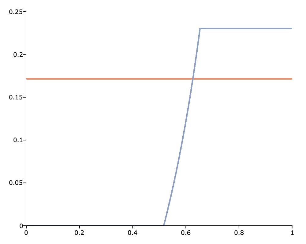
If we draw the graph, using our previous styling and a formula string as shown below:

plotXY(plt, int_rate, "high + low ~ x");

we get the following plot:

Add Vertical Lines

Line styling

We will continue with the plotControl structure we created earlier and modify the line settings to match the vertical lines from the graph we are trying to reproduce.

// Set lines to be: 1 pixel wide, light gray (#CCC) and dashed style (2)
plotSetLinePen(&plt, 1, "#CCC", 2);

Draw the lines

We add the vertical lines using plotAddVLine. plotAddVLine takes an optional plotControl structure as the first input and then a vector of one or more x-axis locations at which to draw the vertical spanning lines.

// The x-axis locations for the vertical lines
ks = { 0.517, 0.653, 0.781 };

plotAddVLine(plt, ks);

Add Text Annotations

Style text boxes

The annotation styling functions use a plotAnnotation structure but work very similarly to the main plot styling (plotSet) functions. Therefore, we will just use comments to describe their actions.

struct plotAnnotation ant;
ant = annotationGetDefaults();

// Set text to be interpreted as LaTeX
annotationSetTextInterpreter(&ant, "latex");

// Turn off the text box bounding line, by setting:
//     line-width=0, line-color="" (ignore), line-style=-1 (no line)
annotationSetLinePen(&ant, 0, "", -1);

// Leave the font-family as default, "",
// Set the font-size to 14 points and the color to a
// dark gray, #333
annotationSetFont(&ant, "", 14, "#3333");

// Leave the annotation background color, "".
// Set the opacity to 0% (100% transparent)
annotationSetBkd(&ant, "", 0);

Draw the text boxes

After the optional plotAnnotation structure, plotAddTextbox takes 3 input arguments:

1. The text to display.
   
2. The x-axis coordinate.
   
3. The y-axis coordinate.
   

By default, the x and y-axis coordinates specify the location of the top-left of the bounding box that contains the text.

plotAddTextbox(ant, "\\omega_1", ks[1], 0.15);
plotAddTextbox(ant, "\\omega_2", ks[2], 0.15);
plotAddTextbox(ant, "\\omega_3", ks[3], 0.15);

Full code

Below is the full code to create our graph.

new;
cls;

/*
** Load and preview data
*/
int_rate = loadd("int_rate.csv");

tail(int_rate);

ks = { 0.517, 0.653, 0.781  };

/*
** Graph data
*/

// Graph size
plotCanvasSize("px", 500 | 400);

// Default settings
struct plotControl plt;
plt = plotGetDefaults("xy");

// Font
plotSetFonts(&plt, "all", "roboto", 14);

// Legend
plotSetLegend(&plt, "", "vcenter left inside", 1);
plotSetLegendBkd(&plt, 0);

// Main line settings
clrs = getColorPalette("set2");
plotSetLinePen(&plt, 4, clrs[3 2], 1|3);

// Axes outline (spine)
plotSetOutlineEnabled(&plt, 1);

// X-axis
plotSetTextInterpreter(&plt, "latex", "xaxis");
plotSetXAxisLabel(&plt, "\\text{country opacity }, \\omega");

// Draw main plot
plotXY(plt, int_rate, "high + low ~ x");

// Style and add vertical lines
plotSetLinePen(&plt, 1, "#CCC", 2);
plotAddVLine(plt, ks);

// Style text boxes
struct plotAnnotation ant;
ant = annotationGetDefaults();
annotationSetTextInterpreter(&ant, "latex");
annotationSetLinePen(&ant, 0, "", -1);
annotationSetFont(&ant, "", 14, "#3333");
annotationSetBkd(&ant, "", 0);

// Add text boxes
plotAddTextbox(ant, "\\omega_1", ks[1], 0.15);
plotAddTextbox(ant, "\\omega_2", ks[2], 0.15);
plotAddTextbox(ant, "\\omega_3", ks[3], 0.15);

Bonus Content: Text Box Anchor Position

For this case, we wanted the text boxes to appear to just the right of the vertical lines and the vertical position of the text boxes was not critical. Therefore, the default anchor position worked well.

However, if we had needed the text boxes to be towards the bottom of the graph, the first of them would have overlapped with one of our lines. We can see this by changing the plotAddTextbox lines to the following:

// Draw the text boxes at a lower position, y=0.04
plotAddTextbox(ant, "\\omega_1", ks[1], 0.04);
plotAddTextbox(ant, "\\omega_2", ks[2], 0.04);
plotAddTextbox(ant, "\\omega_3", ks[3], 0.04);

This makes the bottom of our graph look like this:

In this case, it would be nice to move the text boxes to the left of the vertical line. We can do this by using the final optional input of plotAddTextbox. It is a string that allows you to specify the position of the text box with respect to its anchor position.

The string options include:

• Vertical position: "top", "vcenter", "bottom".
  
• Horizontal position: "left", "hcenter", "right".
  

or "center" which is equivalent to "vcenter hcenter".

For this example, we will just move the text boxes to the left of the vertical lines which are at the same position as the text box's anchor locations:

// Draw the text boxes at a lower position, y=0.04
plotAddTextbox(ant, "\\omega_1", ks[1], 0.04, "left");
plotAddTextbox(ant, "\\omega_2", ks[2], 0.04, "left");
plotAddTextbox(ant, "\\omega_3", ks[3], 0.04, "left");

This gives us the following image:

Conclusion

Great job! You have learned how to:

1. Add and style text boxes with LaTeX.
2. Set the anchor point of text boxes.
3. Add and style vertical lines.
4. Automatically set legend text to use your dataframe's variable names.
5. Set the font for all or a subset of the graph text elements.
6. Set the size of your graph.
7. Control the position of text boxes with respect to their attachment point.

Further Reading

1. Visualizing COVID-19 Data with GAUSS 22
2. How to Mix, Match, and Style Different Graph Types
3. How to Create Tiled Graphs in GAUSS
4. Five Hacks for Creating Custom GAUSS Graphics

References

Farboodi, Maryam, and Péter Kondor. 2022. "Heterogeneous Global Booms and Busts." American Economic Review, 112 (7): 2178-2212. DOI: 10.1257/aer.20181830