Introduction
Anyone who works with panel data knows that pivoting between long and wide form, though commonly necessary, can still be painstakingly tedious, at best. It can lead to frustrating errors, unexpected results, and lengthy troubleshooting, at worst.
The new dfLonger and dfWider procedures introduced in GAUSS 24 make great strides towards fixing that. Extensive planning has gone into each procedure, resulting in comprehensive but intuitive functions.
In today's blog, we will walk through all you need to know about the dfLonger procedure to tackle even the most complex cases of transforming wide form panel data to long form.
The Rules of Tidy Data
Before we get started, it will be useful to consider what makes data tidy (and why tidy data is important).
It's useful to think of breaking our data into components (these subsets will come in handy later when working with dflonger):
- Values.
- Observations.
- Variables.
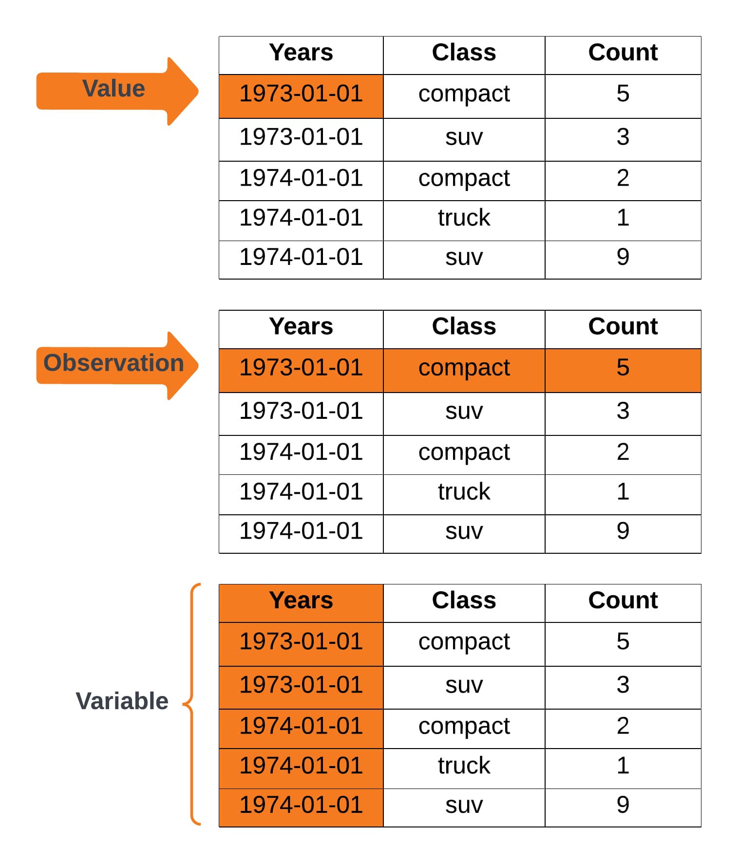
We can use these components to define some basic rules for tidy data:
- Variables have unique columns.
- Observations have unique rows.
- Values have unique cells.
Example One: Wide Form State Population Table
| State | 2020 | 2021 | 2022 |
|---|---|---|---|
| Alabama | 5,031,362 | 5,049,846 | 5,074,296 |
| Alaska | 732,923 | 734,182 | 733,583 |
| Arizona | 7,179,943 | 7,264,877 | 7,359,197 |
| Arkansas | 3,014,195 | 3,028,122 | 3,045,637 |
| California | 39,501,653 | 39,142,991 | 39,029,342 |
Though not clearly labeled, we can deduce that this data presents values for three different variables: State, Year, and Population.
Looking more closely we see:
- State is stored in a unique column.
- The values of Years are stored as column names.
- The values of Population are stored in separate columns for each year.
Our variables do not each have a unique column, violating the rules of tidy data.
Example Two: Long Form State Population Table
| State | Year | Population |
|---|---|---|
| Alabama | 2020 | 5,031,362 |
| Alabama | 2021 | 5,049,846 |
| Alabama | 2022 | 5,074,296 |
| Alaska | 2020 | 732,923 |
| Alaska | 2021 | 734,182 |
| Alaska | 2022 | 733,583 |
| Arizona | 2020 | 7,179,943 |
| Arizona | 2021 | 7,264,877 |
| Arizona | 2022 | 7,359,197 |
The transformed data above now has three columns, one for each variable State, Year, and Population. We can also confirm that each observation has a single row and each value has a single cell.
Transforming the data to long form has resulted in a tidy data table.
Why Do We Care About Tidy Data?
Working with tidy data offers a number of advantages:
- Tidy data storage offers consistency when trying to compare, explore, and analyze data whether it be panel data, time series data or cross-sectional data.
- Using columns for variables is aligned with vectorization and matrix notation, both of which are fundamental to efficient computations.
- Many software tools expect tidy data and will only work reliably with tidy data.
Transforming From Wide to Long Panel Data
In this section, we will look at how to use the GAUSS procedure dfLonger to transform panel data from wide to long form. This section will cover:
- The fundamentals of the
dfLongerprocedure. - A standard process for setting up panel data transformations.
The dfLonger Procedure
The dfLonger procedure transforms wide form GAUSS dataframes to long form GAUSS dataframes. It has four required inputs and one optional input:
df_long = dfLonger(df_wide, columns, names_to, values_to [, pctl]);- df_wide
- A GAUSS dataframe in wide panel format.
- columns
- String array, the columns that should be used in the conversion.
- names_to
- String array, specifies the variable name(s) for the new column(s) created to store the wide variable names.
- value_to
- String, the name of the new column containing the values.
- pctl
- Optional, an instance of the
pivotControlstructure used for advanced pivoting options.
Setting Up Panel Data Transformations
Having a systematic process for transforming wide panel data to long panel data will:
- Save time.
- Eliminate frustration.
- Prevent errors.
Let's use our wide form state population data to work through the steps.
Step 1: Identify variables.
In our wide form population table, there are three variables: State, Year, and Population.
Step 2: Identify columns to convert.
The easiest way to determine what columns need to be converted is to identify the "problem" columns in your wide form data.
For example, in our original state population table, the columns named 2020, 2021, 2022, represent our Year variable. They store the values for the Population variable.
![]()
These are the columns we will need to address in order to make our data tidy.
columns = "2020"$|"2021"$|"2022";We only have three columns to transform and it is easy to just type out our column names in a string array. This won't always be the case, though. Fortunately, GAUSS has a lot of great convenience functions to help with creating your column lists.
My favorites include:
| Function | Description | Example |
|---|---|---|
| getColNames | Returns the column variable names. |
varnames = getColNames(df_wide) |
| startsWith | Returns a 1 if a string starts with a specified pattern. |
mask = startsWith(colNames, pattern) |
| trimr | Trims rows from the top and/or bottom of a matrix. |
names = trimr(full_list, top, bottom) |
| rowcontains | Returns a 1 if the row contains the data specified by the needle variable, otherwise it returns a 0. |
mask = rowcontains(haystack, needle) |
| selif | Selects rows from a matrix, dataframe or string array, based upon a vector of 1’s and 0’s. |
names = rowcontains(full_list, mask) |
For more complex cases, it useful to approach creating column lists as a two-step process:
- Get all column names using
getColNames. - Select a subset of columns names using a selection convenience functions.
As an example, suppose our state population dataset contains a year column as the first column and the remaining columns contain the populations for 1950-2022. It would be difficult to write out the column list for all years.
Instead we could:
- Get a list of all the column names using
getColNames. - Trim the first name off the list.
// Get all columns names
colNames = getColNames(pop_wide);

// Trim first name `year`
// from top of the name list
colNames = trimr(colNames, 1, 0);
Step 3: Name the new columns for storing names.
The names of the columns being transformed from our wide form data will be stored in a variable specified by the input names_to.
In this case, we want to store the names from the wide data in one new variable called, "Years". In later examples, we will look at how to split names into multiple variables using prefixes, separators, or patterns.
names_to = "Years";Step 4: Name the new columns for storing values.
The values stored in the columns being transformed will be stored in a variable specified by the input values_to.
For our population table, we will store the values in a variable named "Population".
values_to = "Population";Basic Pivoting
Now it's time to put all these steps together into a working example. Let's continue with our state population example.
We'll start by loading the complete state population dataset from the state_pop.gdat file:
// Load data
pop_wide = loadd("state_pop.gdat");

// Preview data
head(pop_wide);
State 2020 2021 2022
Alabama 5031362.0 5049846.0 5074296.0
Alaska 732923.00 734182.00 733583.00
Arizona 7179943.0 7264877.0 7359197.0
Arkansas 3014195.0 3028122.0 3045637.0
California 39501653. 39142991. 39029342.
Now, let's set up our information for transforming our data:
// Identify columns
columns = "2020"$|"2021"$|"2022";

// Variable for storing names
names_to = "Year";

// Variable for storing values
values_to = "Population";
Finally, we'll transform our data using df_longer:
// Convert data using df_longer
pop_long = dfLonger(pop_wide, columns, names_to, values_to);

// Preview data
head(pop_long);
State Year Population
Alabama 2020 5031362.0
Alabama 2021 5049846.0
Alabama 2022 5074296.0
Alaska 2020 732923.00
Alaska 2021 734182.00
Advanced Pivoting
One of the most appealing things about dfLonger is that while simple to use, it offers tools for tackling the most complex cases. In this section, we'll cover everything you need to know for moving beyond basic pivoting.
The pivotControl Structure
The pivotControl structure allows you to control pivoting specifications using
the following members:
| Member | Purpose |
|---|---|
| names_prefix | A string input which specifies which characters, if any, should be stripped from the front of the wide variable names before they are assigned to a long column. |
| names_sep_split | A string input which specifies which characters, if any, mark where the names_to names should be broken up. |
| names_pattern_split | A string input containing a regular expression specifying group(s) in names_to names which should be broken up. |
| names_types | A string input specifying data types for the names_to variable. |
| values_drop_missing | Scalar, is set to 1 all rows with missing values will be removed. |
pivotControl structure in later examples. However, if you are unfamiliar with structures you may find it useful to review our tutorial, "A Gentle Introduction to Using Structures."Changing Variable Types
By default the variables created from the pieces of the variable names will be categorical variables.
If we examine the variable type of pop_long from our previous example,
// Check the type of the 'Year' variables
getColTypes(pop_long[., "Year"]);
we can see that the Year variable is a categorical variable:
            type
        category
This isn't ideal and we'd prefer our Year variable to be a date.
We can control the assigned type using the names_types member of the pivotControl structure. The names_types member can be specified in one of two ways:
- As a column vector of types for each of the names_to variables.
- An n x 2 string array where the first column is the name of the variable(s) and the second column contains the type(s) to be assigned.
For our example, we wish to specify that the Year variable should be a date but we don't need to change any of the other assigned types, so we will use the second option:
// Declare pivotControl structure and fill with default values
struct pivotControl pctl;
pctl = pivotControlCreate();

// Specify that 'Year' should be
// converted to a date variable
pctl.names_types = {"Year" "date"};
Next, we complete the steps for pivoting:
// Get all column names and remove the first column, 'State'
columns = getColNames(pop_wide);
columns = trimr(columns, 1, 0);

// Variable for storing names
names_to = "Year";

// Variable for storing values
values_to = "Population";
Finally, we call dfLonger including the pivotControl structure, pctl, as the final input:
// Call dfLonger with optional control structure
pop_long = dfLonger(pop_wide, columns, names_to, values_to, pctl);

// Preview data
head(pop_long);
State Year Population
Alabama 2020 5031362.0
Alabama 2021 5049846.0
Alabama 2022 5074296.0
Alaska 2020 732923.00
Alaska 2021 734182.00
Now if we check the type of our Year variable:
// Check the type of 'Year'
getColTypes(pop_long[., "Year"]);
It is a date variable:
  type
  date
Stripping Prefixes
In our previous example, the wide data names only contained the year. However, the column names of a wide dataset often have common prefixes. The names_prefix member of the pivotControl structure offers a convenient way to strip unwanted prefixes.
Suppose that our wide form state population columns were labeled "yr_2020", "yr_2021", "yr_2022":
// Load data
pop_wide2 = loadd("state_pop2.gdat");

// Preview data
head(pop_wide2);
State yr_2020 yr_2021 yr_2022
Alabama 5031362.0 5049846.0 5074296.0
Alaska 732923.00 734182.00 733583.00
Arizona 7179943.0 7264877.0 7359197.0
Arkansas 3014195.0 3028122.0 3045637.0
California 39501653. 39142991. 39029342.
We need to strip these prefixes when transforming our data to long form.
To accomplish this we first need to specify that our name columns have the common prefix "yr":
// Declare pivotControl structure and fill with default values
struct pivotControl pctl;
pctl = pivotControlCreate();

// Specify prefix
pctl.names_prefix = "yr_";
Next, we complete the steps for pivoting:
// Get all column names and remove the first column, 'State'
columns = getColNames(pop_wide2);
columns = trimr(columns, 1, 0);

// Variable for storing names
names_to = "Year";

// Variable for storing values
values_to = "Population";
Finally, we call dfLonger:
// Call dfLonger with optional control structure
pop_long = dfLonger(pop_wide2, columns, names_to, values_to, pctl);

// Preview data
head(pop_long);
State Year Population
Alabama 2020 5031362.0
Alabama 2021 5049846.0
Alabama 2022 5074296.0
Alaska 2020 732923.00
Alaska 2021 734182.00
Splitting Names
In our basic example the only information contained in the names columns was the year. We created one variable to store that information, "Year". However, we may have cases where our wide form data contains more than one piece of information.
In theses case there are two important steps to take:
- Name the variables that will store the information contained in the wide data column names using the names_to input.
- Indicate to GAUSS how to split the wide data column names into the names_to variables.
Names Include a Separator
One way that names in wide data can contain multiple pieces of information is through the use of separators.
For example, suppose our data looks like this:
           State       urban_2020       urban_2021       urban_2022       rural_2020       rural_2021       rural_2022
         Alabama        6558153.0        4972982.0        12375977.        1526791.0        76863.000        7301681.0
          Alaska        21944.000        467051.00        311873.00        710978.00        267130.00        421709.00
         Arizona        1248007.0        6033358.0        1444029.0        8427950.0        1231518.0        5915167.0
        Arkansas        863918.00        913266.00        7000024.0        2150276.0        3941388.0        3954387.0
      California        17255657.        27682794.        63926200.        22245995.        11460196.        24896858.
Now our names specify:
- Whether the population is the urban or rural population.
- The year of the observation.
In this case, we:
- Use the names_sep_split member of the
pivotControlstructure to indicate how to split the names. - Specify a names_to variable for each group created by the separator.
// Load data
pop_wide3 = loadd("state_pop3.gdat");

// Declare pivotControl structure and fill with default values
struct pivotControl pctl;
pctl = pivotControlCreate();

// Specify how to separate names
pctl.names_sep_split = "_";

// Specify two variables for holding
// names information:
//    'Location' for the information before the separator
//    'Year' for the information after the separator
names_to = "Location"$|"Year";

// Variable for storing values
values_to = "Population";

// Call dfLonger with optional control structure
pop_long = dfLonger(pop_wide3, columns, names_to, values_to, pctl);

// Preview data
head(pop_long);
State Location Year Population
Alabama urban 2020 6558153.0
Alabama urban 2021 4972982.0
Alabama urban 2022 12375977.
Alabama rural 2020 1526791.0
Alabama rural 2021 76863.000
Now, the pop_long dataframe contains:
- The information in the wide form names found before the separator,
"_", (urban or rural) in the Location variable. - The information in the wide form names found after the separator,
"_", in the Year variable.
Variable Names With Regular Expressions
In our example above, the variables contained in the names were clearly separated by a "_". However, this isn't always the case. Sometimes names use a pattern rather than separator:
// Load data
pop_wide4 = loadd("state_pop4.gdat");

// Preview data
head(pop_wide4);
State urban2020 urban2021 urban2022 rural2020 rural2021 rural2022
Alabama 6558153.0 4972982.0 12375977. 1526791.0 76863.000 7301681.0
Alaska 21944.000 467051.00 311873.00 710978.00 267130.00 421709.00
Arizona 1248007.0 6033358.0 1444029.0 8427950.0 1231518.0 5915167.0
Arkansas 863918.00 913266.00 7000024.0 2150276.0 3941388.0 3954387.0
California 17255657. 27682794. 63926200. 22245995. 11460196. 24896858.
In cases like this, we can use the names_pattern_split member to tell GAUSS we want to pass in a regular expression that will split the columns. We can't cover the full details of regular expressions here. However, there are a few fundamentals that will help us get started with this example.
In regEx:
- Each statement inside a pair of parentheses is a group.
- To match any upper or lower case letter we use
"[a-zA-Z]". More specifically, this tells GAUSS that we want to match any lowercase letter ranging from a-z and any upper case letter ranging from A-Z. If we wanted to limit this to any lowercase letters from t to z and any uppercase letter B to M we would say"[t-zB-M]". - To match any integer we use
"[0-9]". - To represent that we want to match one or more instances of a pattern we use
"+". - To represent that we want to match zero or more instances of a pattern we use
"*".
In this case, we want to separate our names so that "urban" and "rural" are collected in Location and 2020, 2021, and 2022 are collected in the Year variable:
- We have two groups.
- We can capture both
urbanandruralusing"[a-zA-Z]+". - We can capture the years by matching one or more number using
"[0-9]+".
Let's use regEx to specify our names_pattern_split member:
// Declare pivotControl structure and fill with default values
struct pivotControl pctl;
pctl = pivotControlCreate();
// Specify how to separate names
// using the pivotControl structure
pctl.names_pattern_split = "([a-zA-Z]+)([0-9]+)"; Next, we can put this together with our other steps to transform our wide data:
// Variable for storing names
names_to = "Location"$|"Year";
// Get all column names and remove the first column, 'State'
columns = getColNames(pop_wide4);
columns = trimr(columns, 1, 0);
// Variable for storing values
values_to = "Population";
// Call dfLonger with optional control structure
pop_long = dfLonger(pop_wide4, columns, names_to, values_to, pctl4);
head(pop_long); State Location Year Population
Alabama urban 2020 6558153.0
Alabama urban 2021 4972982.0
Alabama urban 2022 12375977.
Alabama rural 2020 1526791.0
Alabama rural 2021 76863.000
Multiple Value Variables
In all our previous examples we had values that needed to be stored in one variable. However, it's more realistic that our dataset contains multiple groups of values and we will need to specify multiple variables to store these values.
Let's consider our previous example which used the pop_wide4 dataset:
           State        urban2020        urban2021        urban2022        rural2020        rural2021        rural2022
         Alabama        6558153.0        4972982.0        12375977.        1526791.0        76863.000        7301681.0
          Alaska        21944.000        467051.00        311873.00        710978.00        267130.00        421709.00
         Arizona        1248007.0        6033358.0        1444029.0        8427950.0        1231518.0        5915167.0
        Arkansas        863918.00        913266.00        7000024.0        2150276.0        3941388.0        3954387.0
      California        17255657.        27682794.        63926200.        22245995.        11460196.        24896858.
Suppose that rather than creating a location variable, we wish to separate the population information into two variables, urban and rural. To do this we will:
- Split the variable names by words (
"urban"or"rural") and integers. - Create a Year column from the integer portions of the names.
- Create two values columns, urban and rural, from the word portions.
First, we will specify our columns:
// Get all column names and remove the first column, 'State'
columns = getColNames(pop_wide4);
columns = trimr(columns, 1, 0);Next, we need to specify our names_to and values_to inputs. However, this time we want our values_to variables to be determined by the information in our names.
We do this using ".value".
// Tell GAUSS to use the first group of the split names
// to set the values variables and
// store the remaining group in 'Year'
names_to = ".value" $| "Year";

// Tell GAUSS to get 'values_to' variables from 'names_to'
values_to = "";
Setting ".value" as the first element in our names_to input tells dfLonger to take the first piece of the wide data names and create a column with the all the values from all matching columns.
In other words, combine all the values from the variables urban2020, urban2021, urban2022 into a single variable named urban and do the same for the rural columns.
Finally, we need to tell GAUSS how to split the variable names.
// Declare 'pctl' to be a pivotControl structure
// and fill with default settings
struct pivotControl pctl;
pctl = pivotControlCreate();

// Set the regex to split the variable names
pctl.names_pattern_split = "(urban|rural)([0-9]+)";
This time, we specify the variable names, "(urban|rural)" rather than use the general specifier "([a-zA-Z])".
Now we call dfLonger:
// Convert the dataframe to long format according to our specifications
pop_long = dfLonger(pop_wide4, columns, names_to, values_to, pctl);

// Print the first 5 rows of the long form dataframe
head(pop_long);
State Year urban rural
Alabama 2020 6558153.0 1526791.0
Alabama 2021 4972982.0 76863.000
Alabama 2022 12375977. 7301681.0
Alaska 2020 21944.000 710978.00
Alaska 2021 467051.00 267130.00
Now the urban population and rural population are stored in their own column, named urban and rural.
Conclusion
As we've seen today, pivoting panel data from wide to long can be complicated. However, using a systematic approach and the GAUSS dfLonger procedure help to alleviate the frustration, time, and errors.