Introduction to the Fundamentals of Time Series Data and Analysis

by Eric · Published September 13, 2019 · Updated February 29, 2024

Introduction

Time series data is data that is collected at different points in time. This is opposed to cross-sectional data which observes individuals, companies, etc. at a single point in time.

Because data points in time series are collected at adjacent time periods there is potential for correlation between observations. This is one of the features that distinguishes time series data from cross-sectional data.

Time series data can be found in economics, social sciences, finance, epidemiology, and the physical sciences.

What Is an Example of Time Series Data?
Field	Example topics	Example dataset
Economics	Gross Domestic Product (GDP), Consumer Price Index (CPI), S&P 500 Index, and unemployment rates	U.S. GDP from the Federal Reserve Economic Data
Social sciences	Birth rates, population, migration data, political indicators	Population without citizenship from Eurostat
Epidemiology	Disease rates, mortality rates, mosquito populations	U.S. Cancer Incidence rates from the Center for Disease Control
Medicine	Blood pressure tracking, weight tracking, cholesterol measurements, heart rate monitoring	MRI scanning and behavioral test dataset
Physical sciences	Global temperatures, monthly sunspot observations, pollution levels.	Global air pollution from the Our World in Data

The statistical characteristics of time series data often violate the assumptions of conventional statistical methods. Because of this, analyzing time series data requires a unique set of tools and methods, collectively known as time series analysis.

This article covers the fundamental concepts of time series analysis and should give you a foundation for working with time series data.

What Is Time Series Data?

Time series data is a collection of quantities that are assembled over even intervals in time and ordered chronologically. The time interval at which data is collected is generally referred to as the time series frequency.

For example, the time series graph above plots the visitors per month to Yellowstone National Park with the average monthly temperatures. The data ranges from January 2014 to December 2016 and is collected at a monthly frequency.

Time Series Visualization

What is a time series graph?

A time series graph plots observed values on the y-axis against an increment of time on the x-axis. These graphs visually highlight the behavior and patterns of the data and can lay the foundation for building a reliable model.

More specifically, visualizing time series data provides a preliminary tool for detecting if data:

• Is mean-reverting or has explosive behavior.
• Has a time trend.
• Exhibits seasonality.
• Demonstrates structural breaks.

This, in turn, can help guide the testing, diagnostics, and estimation methods used during time series modeling and analysis.

Mean Reverting Data

Mean reverting data returns, over time, to a time-invariant mean. It is important to know whether a model includes a non-zero mean because it is a prerequisite for determining appropriate testing and modeling methods.

For example, unit root tests use different regressions, statistics, and distributions when a non-zero constant is included in the model.

A time series graph provides a tool for visually inspecting if the data is mean-reverting, and if it is, what mean the data is centered around. While visual inspection should never replace statistical estimation, it can help you decide whether a non-zero mean should be included in the model.

For example, the data in the figure above varies around a mean that lies above the zero line. This indicates that the models and tests for this data must incorporate a non-zero mean.

Time Trending Data

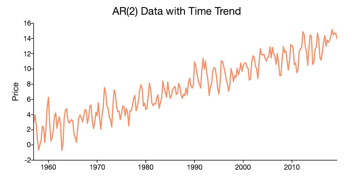
In addition to containing a non-zero mean, time series data may also have a deterministic component that is proportionate to the time period. When this occurs, the time series data is said to have a time trend.

Time trends in time series data also have implications for testing and modeling. The reliability of a time series model depends on properly identifying and accounting for time trends.

A time series plot that looks like it centers around an increasing or decreasing line, like that in the plot above, suggests the presence of a time trend.

Seasonality

Seasonality is another characteristic of time series data that can be visually identified in time series plots. Seasonality occurs when time series data exhibits regular and predictable patterns at time intervals that are smaller than a year.

An example of a time series with seasonality is retail sales, which often increase between September to December and will decrease between January and February.

Structural Breaks

Sometimes time series data shows a sudden change in behavior at a certain point in time. For example, many macroeconomic indicators changed sharply in 2008 after the start of the global financial crisis. These sudden changes are often referred to as structural breaks or non-linearities.

These structural breaks can create instability in the parameters of a model. This, in turn, can diminish the validity and reliability of that model.

Though statistical methods and tests should be used to test for structural breaks, time series plots can help for preliminary identification of structural breaks in data.

Structural breaks in the mean of a time series will appear in graphs as sudden shifts in the level of the data at certain breakpoints. For example, in the time series plot above there is a clear jump in the mean of the data around the start of 1980.

Modeling Time Series Data

Time series models are used for a variety of reasons -- predicting future outcomes, understanding past outcomes, making policy suggestions, and much more. These general goals of time series modeling don’t vary significantly from modeling cross-sectional or panel data. However, the techniques used in time series models must account for time series correlation.

Time-Domain Versus Frequency Domain Models

Two broad approaches have been developed for modeling time series data, the time-domain approach, and the frequency-domain approach.

The time-domain approach models future values as a function of past values and present values. The foundation of this approach is the time series regression of present values of a time series on its own past values and past values of other variables. The estimates of these regressions are often used for forecasting and this approach is popular in time series econometrics.

Frequency domain models are based on the idea that time series can be represented as a function of time using sines and cosines. These representations are known as Fourier representations. Frequency domain models utilize regressions on sines and cosines, rather than past and present values, to model the behavior of the data.

Time Domain Examples	Frequency Domain Examples
Autoregressive Moving Average Models (ARMA)	Spectral analysis
Autoregressive Integrated Moving Average (ARIMA) Models	Band Spectrum Regression
Vector Autoregressive Models (VAR)	Fourier transform methods
Generalized autoregressive conditional heteroscedasticity (GARCH)	Spectral factorization

Univariate Versus Multivariate Time Series Models

Time series models may also be split into univariate time series models and multivariate time series models. Univariate time series models are models used when the dependent variable is a single time series. Trying to model an individual’s heart rate per minute using only past observations of heart rate and exogenous variables is an example of a univariate time series model.

Multivariate time series models are used when there are multiple dependent variables. In addition to depending on their own past values, each series may depend on past and present values of the other series. Modeling U.S. gross domestic product, inflation, and unemployment together as endogenous variables is an example of a multivariate time series model.

Univariate Model Examples	Multivariate Model Examples
Univariate Generalized autoregressive conditional heteroscedasticity (GARCH)	Vector Autoregressive Models (VAR)
Seasonal Autoregressive Integrated Moving Average (SARIMA) Models	Vector Error Correction Model (VECM)
Univariate unit root tests	Multivariate unit root tests

Linear Versus Nonlinear Time Series Models

When structural breaks are present in time series data they can diminish the reliability of time series models that assume the model is constant over time. For this reason, special models must be used to deal with the nonlinearities that structural breaks introduce.

Nonlinear time series analysis focuses on:

• Identifying the presence of structural breaks;
• Estimating the timing of structural breaks;
• Testing for unit roots in the presence of structural breaks;
• Modeling data behavior before, after, and between breaks.

There are different types of nonlinear time series models built around the different natures and characteristics of the nonlinearities. For example, the threshold autoregressive model assumes that jumps in the dependent data are triggered when a threshold variable reaches a specified level. Conversely, Markov-Switching models assume that an underlying stochastic Markov chain drives regime changes.

Real-world Examples of Structural Breaks in Time Series Data
Example	Description
Housing market prices	The concept of a housing bubble gained notoriety after the global financial crash of 2008. Since then much research and theoretical work is being done to identify and predict housing bubbles.
S&P 500 Unconditional Variance	Modeling stock price volatility is crucial to managing financial portfolios. Because of this, much attention is directed toward understanding the underlying behavior of market indicators like the S&P 500.
Global temperatures	Identifying structural breaks in global temperatures has provided support to proponents of global climate change.

Time Series and Stationarity

What does it mean for a time series to be stationary? A time series is stationary when all statistical characteristics of that series are unchanged by shifts in time. In technical terms, strict stationarity implies that the joint distribution of $(y_t, …, y_{t-h})$ depends only on the lag, $h$, and not on the time period, $t$. Strict stationarity is not widely necessary in time series analysis.

This is not to imply that stationarity is not an important concept in time series analysis. Many time series models are valid only under the assumption of weak stationarity (also known as covariance stationarity).

Weak stationarity, henceforth stationarity, requires only that:

• A series has the same finite unconditional mean and finite unconditional variance at all time periods.
• That the series autocovariances are independent of time.

Nonstationary time series are any data series that do not meet the conditions of a weakly stationary time series.

Examples of Stationary Time Series Data

Gaussian White Noise
An example of a stationary time series is a Gaussian white noise process. A Gaussian white noise process is given by

$$ y_t \sim iid N(0, \sigma^2)$$

where $iid$ indicates that the series is independent and identically distributed.

The Gaussian white noise process has a constant mean equal to zero, $E[Y_t]=0$, and a constant variance equal to $\sigma^2$, $Var(Y_t) = \sigma^2$.

Independent White Noise
Independent white noise is any time series data that is drawn from the same distribution with a zero mean and variance $\sigma^2$. An example of an independent white noise series is data drawn from the Student’s t distribution.

Examples of Nonstationary Data

Deterministically Trending Data
When data has a time trend it has a component that is multiplicative with time. For example,

$$y_t = \beta_0 + \beta_1t + \epsilon_t\\ \epsilon_t \sim N(0, \sigma^2)$$

Note that in this case $E[y_t] = \beta_0 + \beta_1t$, which is dependent on $t$.

Data with a time trend is sometimes referred to as a trend stationary time series. This is because it can be transformed into stationary data using a simple detrending process:

$$\tilde{y}_t = y_t - \beta_0 - \beta_1t = \epsilon_t$$

Random Walk
A random walk process is generated when one observation is a random modification of the previous observation. For example,

$$y_t = y_{t-1}+ \epsilon_t$$

Like the deterministically trending data, transforming the random walk data will result in a stationary series:

$$ \Delta y_t = y_t - y_{t-1} = \epsilon_t$$

Time Series and Seasonality

It is important to recognize the presence of seasonality in time series. Failing to recognize the regular and predictable patterns of seasonality in time series data can lead to incorrect models and interpretations.

How to Identify Seasonality

Identifying seasonality in time series data is important for the development of a useful time series model.

There are many tools that are useful for detecting seasonality in time series data:

• Background theory and knowledge of the data can provide insight into the presence and frequency of seasonality.
• Time series plots such as the seasonal subseries plot, the autocorrelation plot, or a spectral plot can help identify obvious seasonal trends in data.
• Statistical analysis and tests, such as the autocorrelation function, periodograms, or power spectrums can be used to identify the presence of seasonality.

Dealing With Seasonality in Time Series Data

Once seasonality is identified, the proper steps must be taken to deal with its presence. There are a few options for addressing seasonality in time series data:

• Choose a model that incorporates seasonality, like the Seasonal Autoregressive Integrated Moving Average (SARIMA) models.
• Remove the seasonality by seasonally detrending the data or smoothing the data using an appropriate filter. If the model is going to be used for forecasting, the seasonal component must be included in the forecast.
• Use a seasonally adjusted version of the data. For example, the Bureau of Labor Statistics provides U.S. labor and employment data and offers many series in both seasonally adjusted and not-seasonally adjusted formats.

Time Series Data and Autocorrelation

What is Autocorrelation?

In time series data, autocorrelation is the correlation between observations of the same dataset at different points in time. The need for distinct time series models stems in part from the autocorrelation present in time series data.

Real-world Examples of Autocorrelation
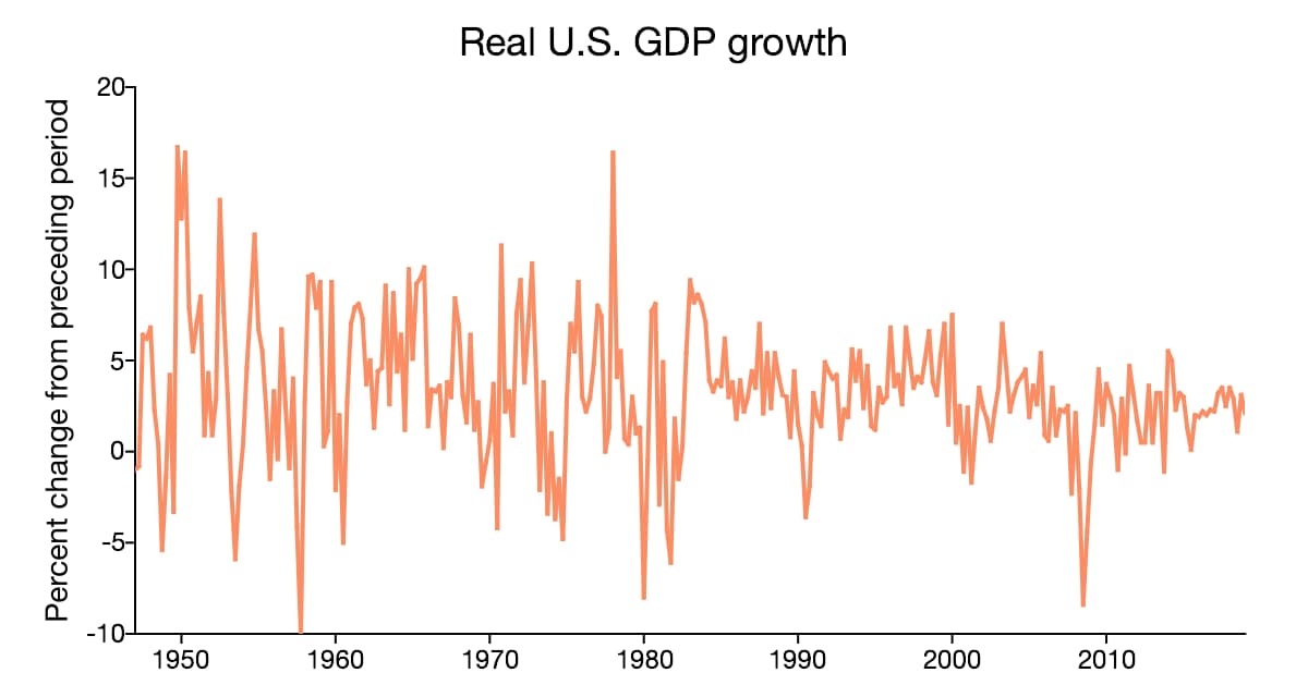
Example	Plot
United States real GDP growth
Luteinizing hormone
Financial time series

What Are the Consequences of Autocorrelation?

Ordinary least squares assumes that there is no autocorrelation in the error terms of a series. When autocorrelation is present, as it is in time series data:

• OLS estimators are valid.
• Traditional OLS standard errors and tests are no longer valid.

What Should Be Done When Autocorrelation Is Present?

When autocorrelation is present, there are two options for finding robust standard errors. The first approach estimates an OLS model and modifies the standard errors afterward. The Newey-West (1987) method is the standard approach for modifying the OLS standard errors to produce heteroskedastic and autocorrelation consistent standard errors.

The alternative for dealing with autocorrelation in time series data is to re-weight the data prior to estimation. One method for doing this is generalized least squares which applies least squares to data that has been transformed by weights. Generalized least squares requires that the true parameters of autocorrelation be known.

More generally, the true parameters of autocorrelations are unknown and must be estimated using feasible generalized least squares (FGLS). Feasible generalized least squares requires estimation of the covariance matrix.

When the covariance structure is assumed the method is known as weighted least squares. Alternatively, the covariance structure can be estimated using iterative methods.

How to Detect Autocorrelation

Detecting autocorrelation in time series data can be done in a number of ways. One preliminary measure for detecting autocorrelation is a time series graph of residuals versus time. If no autocorrelation is present the residuals should appear random and scattered around zero. If there is a pattern in the residuals present, then autocorrelation is likely.

The Durbin-Watson Test
If the time series plot suggests autocorrelation, then further statistical tests can be used to formally test for autocorrelation.

The Durbin-Watson test is a test of the null hypothesis of no first-order autocorrelation against the alternative that the error term in one period is negatively or positively correlated with the error term in the previous period.

The Durbin-Watson Test:

1. Estimate the model using ordinary least squares.
2. Predict the dependent variable using parameter estimates from Step One.
3. Compute the residuals by subtracted predicted dependent variables from the observed dependent variable.
4. Square and sum the residuals.
5. Compute the difference between the residual at each time period, t, and the previous time period, t-1. Then square the differences, and find the sum.
6. Compute the Durbin-Watson statistic by dividing the sum from Step Five by the sum in Step Four.

Upper and lower critical values for the Durbin-Watson statistic depend on the number of independent variables. The computed Durbin-Watson statistic should be compared to these critical values:

$$d \lt d_l \rightarrow \text{reject the null hypothesis}\\ d \gt d_u \rightarrow \text{do not reject the null hypothesis}\\ d_l \lt d \lt d_u \rightarrow \text{test is inconclusive.}$$

The Bruesch-Godfrey Test
When higher-order autocorrelation is suspected the Durbin-Watson test is not valid and the Breusch-Godfrey test should be used instead.

The Breusch-Godfrey test is a test of the null hypothesis of no q-order autocorrelation against the alternative of q-order autocorrelation.

The Bruesch-Godfrey Test:

1. Estimate the model without lagged variables using ordinary least squares.
2. Predict the dependent variable using parameter estimates from Step One.
3. Compute the residuals by subtracting the predicted dependent variable from the observed dependent variable.
4. Regress the estimated residuals on lagged values of the residuals up to lag q and all the original independent variables.
5. Compute the F-test of the joint significance of the lagged residuals.

If the Bruesch-Godfrey F-test statistic is greater than the critical value then the null hypothesis of no q-order autocorrelation is rejected.

Time Series Technique: The Box-Jenkins ARIMA Method

The Box-Jenkins method for ARIMA modeling is a procedure for consistently identifying, estimating, and evaluating ARIMA models.

What Is an ARIMA Model?

The autoregressive integrated moving average model (ARIMA) is a fundamental univariate time series model. The ARIMA model is made up of three key components:

• The autoregressive component is the relationship between the current dependent variable the dependent variable at lagged time periods.
• The integrated component refers to the use of transforming the data by subtracting past values of a variable from the current values of a variable in order to make the data stationary.
• The moving average component refers to the dependency between the dependent variable and past values of a stochastic term.

The ARIMA data is described by the order of each of these components with the notation ARIMA(p, d, q) where:

• p is the number of autoregressive lags included in the model.
• d is the order of differencing used to make the data stationary.
• q is the number of moving average lags included in the model.

What Is the Box-Jenkins Method for ARIMA Models?

The Box-Jenkins method for estimating ARIMA models is made up of several steps:

1. Transform data so it meets the assumption of stationarity.
2. Identify initial proposals for p, d, and q.
3. Estimate the model using the proposed p, d, and q.
4. Evaluate the performance of the proposed p, d, and q.
5. Repeat steps 2-4 as needed to improve model fit.

Transforming the Data for Stationarity

The first step of the Box-Jenkins model involves:

1. Performing unit root tests to confirm the stationarity of the time series data.
2. Taking the proper order of differencing in the case that the raw data is not stationary.
3. Retesting for stationarity after the data has been differenced.

How to Identify the Order of an ARIMA Model

Identifying the autoregressive and moving average orders of the ARIMA model can be done using a variety of statistical tools:

• Patterns in the autocorrelation function (ACF) and the partial autocorrelation function (PACF).
• The Box-Pierce and Box-Ljung tests of joint significance of autocorrelation coefficients.
• The Akaike information criterion (AIC) and Bayesian (Schwarz) criterion (BIC or SIC).

What Are the Methods for Estimating ARIMA Models?

Techniques for ARIMA model include:

• Least squares nonlinear and linear regression.
• Maximum likelihood methods.
• Generalized method of moments.

What Diagnostics Should Be Performed on an ARIMA model?

Once an ARIMA model is estimated the performance of that model should be evaluated using statistical diagnostics. The residuals of the model should be closely examined using tools like:

• The Q-Q plot for comparing the distribution of errors to the normal distribution.
• ACF and PACF plots.
• The Box-Ljung LM test.

Time Series Technique: The VAR Model

Multivariate time series analysis provides insight into the interactions and comovements of a group of time series variables. For example, a multivariate time series model may study the comovement of temperature, wind speed, and precipitation.

The most common multivariate time series model is known as the VARMA model. The VARMA model is analogous to the ARIMA model and contains an autoregressive component and a moving average component.

In the multivariate model, the moving average component is uncommon and the more common case is the pure vector autoregressive model (VAR).

The VAR model is a flexible model that has shown great success in forecasting and has been used for policy and structural analysis.

What Is the Vector Autoregressive Model?

The vector autoregressive model represents a group of dependent time series variables as combinations of their own past values and past values of the other variables in the group.

For example, consider a trivariate model of the relationship between hourly temperature, wind speeds, and precipitation. This model describes the relationship for all three variables, temperature, wind speeds and precipitation as functions of the past values:

$$temp_t = \beta_{11}temp_{t-1} + \beta_{12}wind_{t-1} + \beta_{13}prec_{t-1}$$ $$prec_t = \beta_{21}temp_{t-1} + \beta_{22}wind_{t-1} + \beta_{23}prec_{t-1}$$ $$wind_t = \beta_{31}temp_{t-1} + \beta_{32}wind_{t-1} + \beta_{33}prec_{t-1} $$

Cross-covariance and Cross-correlation Functions

Two key characteristics of the univariate time series model are the autocorrelation function and the covariance. The autocorrelation function measures the correlation of a univariate series with its own past values. The covariance measure the joint variability of the dependent time series with other variables.

The analogies of these in the multivariate time series model are the cross-covariance and the cross-correlation. These measures provide insight into how the individual series in a group of time series are related.

What Is the Cross-correlation Function?
The time series cross-correlation function measures the correlation between one series at various points in time with the values in another series at various points in time.

The cross-correlation function:

• Is scaled with values between -1 and 1;
• Measures how strongly two time series are related;
• Shows how the relationship between variables changes across time.

For example, the cross-correlation function between the temperatures and wind speeds observed at 8:00 am, 9:00 am, and 10:00 gives:

1. The correlation of the temperatures at 8:00 am with the wind speeds at 8:00 am, 9:00 am and 10:00 am.
2. The correlation of the temperatures at 9:00 am with the wind speeds at 8:00 am, 9:00 am and 10:00 am.
3. The correlation of the temperatures at 10:00 am with the wind speeds at 8:00 am, 9:00 am, and 10:00 am.

What Is the Cross-covariance Function?
The time series cross-covariance measures the covariance between values in one time series with values of another time series.

The cross-covariance function:

• Is an unscaled measure;
• Reflect the direction and scale of comovement between two series.

How to Estimate a VAR Model

An unrestricted VAR model is composed of $K$ equations, one for each of the time series variables in the group. Assuming that the VAR model is

• Stationary,
• Has the same regressors,
• Has no restrictions on the parameters,

each individual equation in the VAR model can be estimated using ordinary least squares.

Like ARIMA models, VAR models may also be estimated using the generalized method of moments or maximum likelihood.

Lag Selection in VAR Models

Like the univariate model, one of the important steps of the VAR model is to determine the optimal lag length.

The optimal lag length selection for VAR models is based on information criterion such as the:

• Akaike information criterion (AIC).
• Bayesian (Schwarz) criterion.
• Hannan-Quinn (HQ) information criterion.

Time Series Applications

Time series analysis has many real-world applications. This section looks at several real-world cases for applying time series models.

New York Stock Exchange Closing Values

The NYSE composite adjusted closing price is an example of a univariate time series with potential autocorrelation. The Box-Jenkins method can be used to fit an appropriate ARIMA model to the data.

Testing for Stationarity
Though the time series graph of the NYSE composite adjusted closing price suggests that the series is stationary, statistical tests should be used to confirm this.

This example uses the Augmented Dickey-Fuller unit root test and the Generalized Dickey-Fuller unit root test, both in the GAUSS Time Series MT library.

library tsmt;

// Load data
nyse = loadd("nyse_closing.xlsx", "adj_close");

// Transform to percent change
ch_nyse = (nyse[1:rows(nyse)-1] - nyse[2:rows(nyse)]) ./ nyse[2:rows(nyse)];

/*
** Unit root testing
*/

// Augmented Dickey-Fuller test
p = 0;
l = 3;
{ alpha, tstat_adf, adf_t_crit } = vmadfmt(nyse, p, l);
print "tstat_adf"; tstat_adf;
print "adf_t_crit"; adf_t_crit;

// GLS Dickey-Fuller test
trend = 0;
maxlag = 12;
{ tstat_gls, zcrit } = dfgls(nyse, maxlag, trend);
print "tstat_gls"; tstat_gls;
print "zcrit"; zcrit;

The Augmented Dickey-Fuller test statistic is -2.0849669 which suggests that the null hypothesis of a unit root cannot be rejected at the 10% level.

Similarly, the GLS Dickey-Fuller test statistic is -1.6398621 which confirms that the null hypothesis of a unit root cannot be rejected at the 10% level.

Based on these results the first differences of the data will be used.

The PACF and ACF Functions
The autocorrelation function and partial autocorrelation functions provide guidance for what autoregressive order and moving average order are appropriate for our model.

The ACF and PACF functions can be computed using the lagReport GAUSS function provided in the TSMT library.

/*
** PACF and ACF testing
*/
// Maximum number of autocorrelations
k = 12;

// Order of differencing
d = 1;

// Compute and plot the sample autocorrelations
{ acf_nyse, pacf_nyse } = lagreport (nyse, k, d);

The lagReport function provide ACF and PACF plots:

The ACF and PACF falls below the significance line at all lag values (blue dotted line) in these graphs. This suggests that there is no autocorrelation in the series.

Estimate the ARIMA Model
Despite the results of the PACF and ACF, the ARIMA model will be estimated using the arimaFit procedure in GAUSS for demonstration:

/*
** Estimate the ARIMA(1,1,0) model
*/
call arimaFit(nyse, 1, 1, 0);

This prints the output:

Log Likelihood:   2091.560130         Number of Residuals: 250
AIC           :  -4181.120259         Error Variance     : 11768.138992177
SBC           :  -4177.598798         Standard Error     : 108.481053609

DF: 249      SSE: 2930266.609052175

Coefficients       Std. Err.   T-Ratio    Approx. Prob.
AR[1,1] 0.01905    0.06339     0.30055    0.76401

Constant:  -1.15163318

Unsurprisingly, the AR(1) coefficient is not statistically significant, as suggested by its low t-ratio and the high p-value. This is consistent with the ACF and PACF and confirms the conclusion that the ARIMA model is not the appropriate model for the NYSE composite adjusted closing price.

U.S. Wholesale Price Index (1960q1 - 1990q4)

The U.S Wholesale Price Index is a classic time series dataset that has been used to demonstrate the Box-Jenkins method (See Enders 2004).

Testing for Stationarity
Unlike the NYSE composite adjusted closing price, the time series plot of the WPI suggests that the level series might be nonstationary.

Using the Augmented Dickey-Fuller and the Generalized Dickey-Fuller unit root tests will help confirm this. This time, a trend is included in the test because of the apparent trend in the time series plot of the data:

library tsmt;

// Load the variable 'ln_wpi' from the dataset
wpi = loadd("wpi1.dat", "ln_wpi");

// Transform to percent change
ch_wpi = (wpi[1:rows(wpi)-1] - wpi[2:rows(wpi)]) ./ wpi[2:rows(wpi)] * 100;

/*
** Unit root testing on level data
*/

// Augmented Dickey-Fuller test
p = 1;
l = 3;
{ alpha, tstat_adf, adf_t_crit } = vmadfmt(wpi, p, l);
print "Unit root ADF test results : tstat_adf"; tstat_adf;
print "Unit root ADF test results : adf_t_crit"; adf_t_crit;

// GLS Dickey-Fuller test
trend = 1;
maxlag = 12;
{ tstat_gls, zcrit } = dfgls(wpi, maxlag, trend);
print "Unit root GLS-ADF test results : tstat_gls"; tstat_gls;
print "Unit root GLS-ADF test results : zcrit"; zcrit;

The Augmented Dickey-Fuller test statistic is -2.250 which suggests that the null hypothesis of a unit root cannot be rejected at the 10% level. Similarly, the GLS Dickey-Fuller test statistic is -1.627 which confirms that the null hypothesis of a unit root cannot be rejected at the 10% level. Both of these findings provide evidence that the data may not be stationary.

Based on these results the first differences of the data will be used and a unit root test on the differenced data is performed:

/*
** Unit root testing on percent change data
*/

// Augmented Dickey-Fuller test
p = -1;
l = 3;
{ alpha, tstat_adf, adf_t_crit } = vmadfmt(ch_wpi, p, l);
print "Unit root ADF test results ch_wpi: tstat_adf"; tstat_adf;
print "Unit root ADF test results ch_wpi: adf_t_crit"; adf_t_crit;

// GLS Dickey Fuller test
trend = 0;
maxlag = 12;
{ tstat_gls, zcrit } = dfgls(ch_wpi, maxlag, trend);
print "Unit root GLS-ADF test results ch_wpi: tstat_gls"; tstat_gls;
print "Unit root GLS-ADF test results ch_wpi: zcrit"; zcrit;

Now both the Augmented Dickey-Fuller, -1.546, and the GLS Dickey-Fuller test, -1.606, are closer to suggesting that the null hypothesis of a unit root can be rejected at the 10% level. However, the tests cannot completely allow for the rejection of the unit root null hypothesis.

Why didn't differencing solve the nonstationarity? This may suggest the presence of seasonality or a structural break in the data.

One source of nonstationarity may be a change in volatility, which is suggested in the time series plot in the bottom panel. This could be statistically examined using tests for structural changes in volatility.

The PACF and ACF Functions
The ACF and PACF functions can be computed using the lagReport GAUSS function provided in the TSMT library.

/*
** PACF and ACF testing
*/
// Maximum number of autocorrelations
k = 12;

// Order of differencing
d = 0;

// Compute and plot the sample autocorrelations
{ acf_wpi, pacf_wpi } = lagreport(ch_wpi, k, d);

The lagReport function provide ACF and PACF plots:

The ACF and PACF clearly show significant values.

There are a few notable patterns in the WPI ACF and PACF that can help choose preliminary orders for the ARIMA model:

1. The PACF shows a sharp cut-off after 2 lags (though there is a spike at the fourth lag which may indicate some seasonality).
2. The ACF function shows a slower, more gentle decline. This is sometimes referred to as a geometric pattern.

The combination of the two features above is indicative of an AR(2) model. There are more general patterns in the combination of the ACF and PACF plots that be used to identify the order of ARIMA models:

	ACF	PACF
AR model	Geometric decline.	Sharp loss of significance at p lags.
MA model	Sharp loss of significance at q lags.	Geometric decline.
ARMA model	Geometric decline.	Geometric decline.

Estimate the ARIMA Model
Despite the results of unit root tests, the ARIMA model will be estimated for demonstration. Based on the results of the PACF and ACF an ARIMA(2,1,0) model is estimated using the arimaFit procedure in GAUSS:

/*
** Estimate the arima model
*/
struct arimamtOut aOut;
aOut = arimaFit(wpi, 2, 1, 0);

This prints the output:

Log Likelihood:   -146.366121         Number of Residuals: 123
AIC           :    296.732242         Error Variance     : 0.000120756
SBC           :    302.356611         Standard Error     : 0.010988925

DF: 121      SSE: 0.014611534

Coefficients      Std. Err.  T-Ratio    Approx. Prob.
AR[1,1] 0.45945   0.08766    5.24154    0.00000
AR[2,1] 0.26237   0.08796    2.98282    0.00346

The t-ratio and the low p-values on both the AR(1) and AR(2) coefficients support the use of the ARIMA(2,1,0) model for the WPI data.

Note that this time arimamtOut structure was used to store the results from the model. The stored results include the residuals which are used next for model diagnostics.

Model Diagnostics
Using the lagReport procedure on the residuals stored in aOut.e shows that most the autocorrelation has been properly removed using the ARIMA(2, 1, 0) model:

// Compute and plot the sample autocorrelations
{ acf_wpi, pacf_wpi } = lagreport(aOut.e, k, d);

There is still significant autocorrelation in the 4th lag which suggests that further exploration of a seasonal filter or model should be performed.

Conclusion

Congratulations! You should now have an in-depth understanding of the fundamentals of time series analysis.

Suggested further reading:

1. How to Conduct Unit Root Tests in GAUSS
2. A Guide to Conducting Cointegration Tests
3. Unit Root Tests with Structural Breaks
4. How to Interpret Cointegration Test Results

To learn more about performing time series analysis using GAUSS contact us for a GAUSS demo copy.