What are structural break models?
Time series models estimate the relationship between variables that are observed over a period of time. Many models assume that the relationship between these variables stays constant across the entire period.
Interactive Structural Break Simulator

However, there are cases where changes in factors outside of the model cause changes in the underlying relationship between the variables in the model. Structural break models capture exactly these cases by incorporating sudden, permanent changes in the parameters of models.
Structural break models can integrate structural change through any of the model parameters. Bai and Perron (1998) provide the standard framework for structural breaks model in which some, but not all, of the model parameters are allowed to break at m possible break points,
$$ y_t = x_t' \beta + z_t' \delta_j + u_t $$
$$ t = T_{j-1} + 1, \ldots , T ,$$
where $j = 1, \ldots, m+1$. The dependent variable $y_t$ is to be modeled as a linear combination of regressors with both time invariant coefficients, $x_t$, and time variant coefficients, $z_t$.
Alternatively, the variance break model assumes that breaks occur in the variance of the error term such that
$$ y_t = x_t' \beta + u_t ,$$ $$ var(u_t) = \sigma_1^2,~ t ≤ T_1 ,$$ $$ var(u_t) = \sigma_2^2,~ t > T_1 .$$
Why should I worry about structural breaks?
"Structural change is pervasive in economic time series relationships, and it can be quite perilous to ignore. Inferences about economic relationships can go astray, forecasts can be inaccurate, and policy recommendations can be misleading or worse." -- Bruce Hansen (2001)
Time series models are used for a variety of reasons -- predicting future outcomes, understanding past outcomes, making policy suggestions, and much more. Parameter instability diminishes the ability of a model to meet any of these objectives. Research has demonstrated:
- Many important and widely used economic indicators have been shown to have structural breaks.
- Failing to recognize structural breaks can lead to invalid conclusions and inaccurate forecasts.
- Identifying structural breaks in models can lead to a better understanding of the true mechanisms driving changes in data.
Economic indicators with structural breaks
In a 1996 study, Stock and Watson examine 76 monthly U.S. economic time series relations for model instability using several common statistical tests. The series analyzed encompassed a variety of key economic measures including interest rates, stock prices, industrial production, and consumer expectations. The complete group of variables studied was chosen by the authors to meet four criteria:
- The sample included important monthly economic aggregates and coincident indicators.
- The sample included important leading indicators.
- The series represented a number of different types of variables, spanning different time series properties.
- The variables had consistent historical definitions or adjustments could easily be made if definitions changed over time.
In this study Stock and Watson find evidence that a "substantial fraction of forecasting relations are unstable." Based on this finding the authors make several observations:
- Systematic stability analysis is an important part of modeling.
- Failure to appropriate model "commonplace" instability in models, "calls into question the relevance of policy implications".
- There is an opportunity to improve on the forecasts made by fixed-parameter models.
Rossi (2013) updates the data in this study to include data through 2000 and comes to the same conclusions that, there is clear empirical evidence of instabilities and that these instabilities impact forecast performance.
Other studies find evidence for structural breaks in models of a number of economic and financial relationships including:
- International real interest rates and inflation (Rapach and Wohar, 2005)
- The equity premium (Kim, Morley and Nelson, 2005)
- Global house prices (Knoll, Schularick and Steger, 2014)
- CO2 emissions (Acarvci and Erdogan, 2016)
- The monetary policy reaction function (Inoue and Rossi, 2011).
Forecast performance and structural breaks
In the same 1996 study, Stock and Watson examine the impacts structural breaks can have on forecasting when not properly included in a model. In particular, the study compares the forecast performance of fixed-parameter models to models that allow parameter adaptivity including recursive least squares, rolling regressions, and time-varying parameter models.
The study finds that in over half of the cases the adaptive models perform better than the fixed-parameter models based on their out-of-sample forecast error. The bottom line is that failing to account for structural changes leads results in model misspecification which in turn leads to poor forecast performance.
"The potential empirical importance of departures from constant parameter linear models is undeniable" -- Koop and Potter (2011)
A number of studies following this work have found similar results, showing that structural breaks can impact forecast performance. In their 2011 paper, Pettenuzzo and Timmermann show that including structural breaks in asset allocation models can improve long-horizon forecasts and that ignoring breaks can lead to large welfare losses. Inoue and Rossi (2011) show the importance of identifying parameter instabilities for improving the performance of DSGE models.
When should I consider structural break models?
Structural breaks aren’t right for all data and knowing when to use them is important for building valid models. While there are statistical tests for structural breaks, which we discuss in the next section, there are some preliminary checks that help determine when you may need to consider structural breaks.
Visual plots indicate a change in behavior
Time series plots provide a quick, preliminary method for finding structural breaks in your data. Visually inspecting your data can provide important insight into potential breaks in the mean or volatility of a series. Don’t forget to examine both independent and dependent variables as sudden changes in either can change the parameters of a model.


Poor out-of-sample forecasts
Structural breaks in a model serve as one possible reason for poor forecast performance. A fixed parameter model cannot be expected to forecast well if the true parameters of the model change over time. Conversely, if your model isn't forecasting well, it may be worth considering if model instabilities could be playing a role.
"Why do instabilities matter for forecasting? Clearly, if the predictive content is not stable over time, it will be very difficult to exploit it to improve forecasts"
Theoretical support for model change
There are many cases where economic theory suggests that there should be a change in a modeled relationship. In the cases that economic theory, or even economic intuition, points towards structural breaks the possibility should be considered.

In some cases these changes may be widely acknowledged such as the change in volatility of a number of key economic indicators around the mid-1980s, known as "The Great Moderation", the decline in economic growth between 2007-2009 during the "Great Recession", and sudden changes in policy stances such as the "Volcker Rule" and "Zero lower bound" (Giacomini and Rossi, 2011).
Beyond these, there could be a number of reasons for changes in models over time including legislative or regulatory changes, technological changes, institutional changes, changes in monetary or fiscal policy, or oil price shocks.
What statistical tests are there for identifying structural breaks?
Testing for structural breaks is a rich area of research and there is no one-size-fits-all test for structural breaks and which test to implement depends on several factors. Is the break date known or unknown? Is there a single break or multiple breaks?
Knowing the statistical characteristics of both the breaks and your data help to ensure that the correct test is implemented. Below we highlight some of the classic tests that have shaped the field of structural break testing.
The Chow Test
The Chow (1960) test was one of the first tests which set the foundation for structural break testing. It is built on the theory that if parameters are constant then out-of-sample forecasts should be unbiased. It tests the null hypothesis that there is no structural break against the alternative that there is a known structural break at time $T_b$. The test considers a linear model split into samples at a predetermined break point such that
$$ y_{t} = x_{t}'\beta_1 + u_t ,$$
$$ for~ t ≤ T_ b .$$
and
$$ y_{t} = x_{t}'\beta_2 + u_t ,$$
$$ for~ t > T_b .$$
The test estimates coefficients for each period and uses the out-of-sample forecast errors to compute an F-test comparing the stability of the estimated coefficients across the two periods. One key issue with the Chow test is that the break point must be predetermined prior to implementing the test. Furthermore, the break point must be exogenous or the standard distribution of the statistic is not valid.
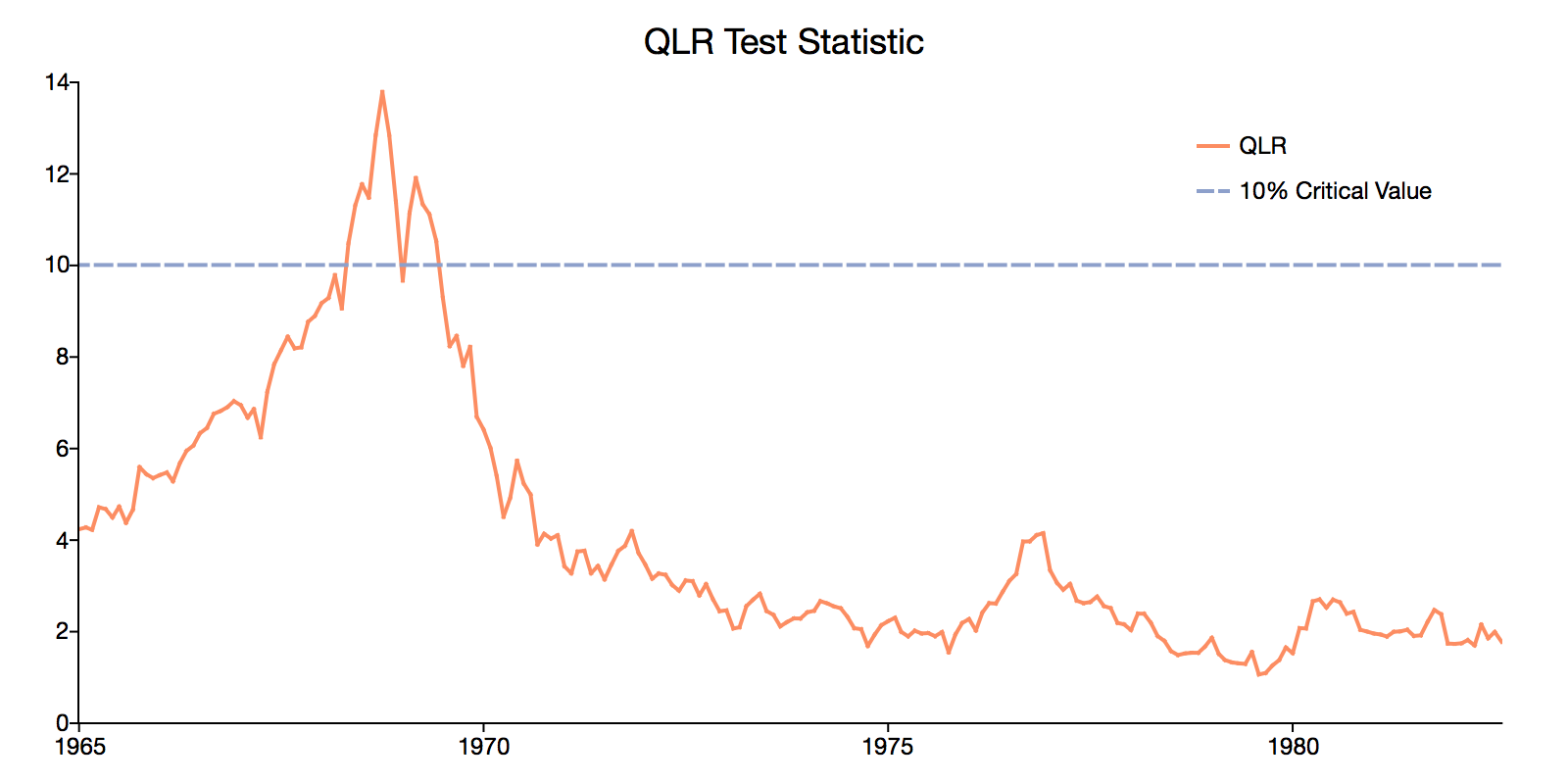
The Quandt Likelihood Ratio Test
The Quandt Likelihood Ratio (QLR) (1960) test builds on the Chow test and attempts to eliminate the need for picking a break point by computing the Chow test at all possible break points. The largest Chow test statistic across the grid of all potential break points is chosen as the Quandt statistic as it indicates the most likely break point.
This test was widely unusable because the limiting distribution of the test statistic under the assumption of an unknown break point was not known. However, the test became statistically relevant when Andrews and Ploberg (1994), developed an applicable distribution for the test-statistic for cases such as the Quandt test.
The CUSUM Test
In their 1975 paper Brown, Durban, and Evans propose the CUSUM test of the null hypothesis of parameter stability. The CUSUM test for instability is appropriate for testing for parameter instability in the intercept term. It is best described as a test for instability of the variance of post-regression residuals.
The CUSUM test is based on the recursive least square estimation of the model
$$ y_t = x_t'\beta_t + u_t $$
for all $k+1 ≤ t ≤ T$. This yields a set of estimates for $\beta$, ${\beta_{k+1}, \beta_{k+2}, \ldots, \beta_T}$. The CUSUM test statistic is computed from the one-step-ahead residuals of the recursive least squares model. It is based on the intuition that if $\beta$ changes from one period to the next then the one-step-ahead forecast will not be accurate and the forecast error will be greater than zero.
This means the greater the CUSUM test statistic, the greater the forecast error, and the greater the statistical evidence in favor of parameter instability.

The Hansen and Nyblom Tests
The Hansen (1992) and Nyblom (1989) tests provide additional Lagrange multiplier parameter stability tests.
-
The Nyblom test, tests the null hypothesis that all parameters are constant against the alternative of that some of the parameters are unstable.
- The Hansen test builds on the Nyblom test to allow for testing constancy in single parameters.
A nice feature of these tests is that they do not require that the model is estimated by OLS. However, unlike the other tests mentioned, neither test provides a mean for identifying the breakpoint.
Comparing parameter stability tests
- Easy to implement.
- F-statistic with standard distribution.
- Must select an *exogenous* break date for $\chi^2$ distribution of statistic to be valid.
- Works with unknown break point.
- Graph of the QLR statistic can provide insight into location of break.
- Non-standard distribution that depends on the number of variables and series trimming.
- Computationally burdensome.
- Recursive residuals can be efficiently computed using Kalman Filter.
- Ploberger and Kramer (1990) show that the OLS CUSUM test statistic can be constructed using the full-sample residuals rather than the recursive residuals.
- Power only in the direction of mean regressors.
- Tests for instability in intercept only.
- Recursive residuals can be efficiently computed using Kalman Filter.
- Has standard $\chi^2(t)$ distribution.
- Power only for changes in variance.
- Tests constancy of all parameters.
- Does not require that model is estimated by OLS.
- Does not provide information about location of break.
- Statistic has non-standard distribution which is dependent on the number of variables.
- Distribution is different if data are non-stationary.
- Tests are easy to compute.
- Tests are robust to heteroscedasticity.
- Individual tests are informative about the type of structural break
- Does not provide information about location of break.
- Statistic has non-standard distribution which is dependent on the number of variables [tested for non-stationarity](https://www.aptech.com/blog/how-to-conduct-unit-root-tests-in-gauss/).
- Distribution is different if data are non-stationary.
How are structural break models estimated?
Structural break models present a number of unique estimation issues that must be considered.
- The location of the structural break in the data is often unknown and therefore must be estimated.
- It must be determined if the model is a pure structural break model, in which all regression parameters change, or a partial structural break model, in which only some of the parameters change.
- The pre and post-break model parameters must be estimated.
The exact method of estimation will depend on the characteristics of your data and the assumptions imposed on the model. However, the general guiding principle of least-squares estimation is similar to that of the model without structural breaks. The number and location of the structural breaks are chosen jointly with the parameters of the model to minimize the sum of the squared error.
Estimation framework
Bai and Perron (1998, 2003) provide the foundation for estimating structural break models based on least squares principles. Bai and Perron start with following multiple linear regression with m breaks
$$ y_t = x_t' \beta + z_t' \delta_j + u_t $$
$$ t = T_{j-1} + 1, \ldots , T ,$$
where $j = 1, \ldots, m+1$. The dependent variable $y_t$ is to be modeled as a linear combination of regressors with both time-invariant coefficients, $x_t$, and time variant coefficients, $z_t$. This model is rewritten in matrix form as
$$ Y = X\beta + \bar{Z}\delta + U $$
where $Y = (y_1, \ldots, y_T)'$, $X = (x_1, \ldots, x_T)'$, $U = (u_1, \ldots, u_T)'$, $\delta = (\delta_1', \ldots, d_{m+1}')'$ and $\bar{Z}$ is a matrix which diagonally partitions Z at $(T_1, \ldots, T_m)$ such that $ \bar{Z} = diag(Z_1, \ldots, Z_{m+1})$.
For each time partition, the [least squares(https://www.aptech.com/resources/tutorials/econometrics/linear-regression/) estimates of $\beta$ and $\delta_j$ are those that minimize
$$ (Y - X\beta - \bar{Z}\delta)'(Y - X\beta - \bar{Z}\delta) = \sum_{i=1}^{m+1} \sum_{t = T_{i-1} + 1}^{T_i} [y_t - x_t'\beta - x_t'\delta_i]^2 $$.
Given the m partitions the estimates become $\hat{\beta}(\{T_j\})$ and $\hat{\delta}(\{T_j\})$. These coefficients and the m partitions are chosen as the global minimizers of the sum of the squared residuals across all partitions
$$ (\hat{T}_1, \ldots, \hat{T}_m) = argmin_{T_1, \ldots, T_m} S_T(T_1, \ldots, T_m) $$
where $ S_T(T_1, \ldots, T_m) $ are the sum of squared residuals given $\hat{\beta}(\{T_j\})$ and $\hat{\delta}(\{T_j\})$
Dynamic programming
The computational burden of estimating both m break points and the period-specific coefficients is quite large. However, Bai and Perron (2003), show that the complexity can be significantly reduced using the concept of dynamic programming.
The dynamic programming algorithm is based on the concept of the Bellman's principle. Given $SSR(\{T_{r,n}\})$, the sum of squared residuals associated with the optimal partition containing r breaks and n observations, the Bellman principle finds that the optimal partitions solve the recursive problem
$$ SSR(\{T_{m,T}\}) = \underset{m = h ≤ j ≤ T-h}{min} [SSR(\{T_{m-1,j}\}) + SSR(j+1,T)] $$
where the sum of squared residuals, $SSR(j,i)$ , is found using the recursive residual, $v(i, j)$, such that
$$ SSR(i, j) = SSR(i, j-1) + v(i,j)^2 $$
This dynamic problem can be solved sequentially first finding the optimal one-break partition, then finding the optimal two-break partitions, and continuing until the optimal $m-1$ partitions are found.
What are some alternatives to structural break models?
Structural break models make a very specific assumption about how changes in model parameters occur. They assume that parameters shift immediately at a specific breakpoint.
This may intuitively make sense when there are distinct and immediate changes in conditions that impact a model. However, there are other models that allow for different manners of parameter shifts.
-
Time-varying parameter models assume that parameters change gradually over time while threshold models assume that model parameters change based on the value of a specified threshold variable.
- Markov-switching models offer an even different solution that assumes that an underlying stochastic Markov chain drives regime changes. Theory and statistical tests should drive the decision of which of these models you use.
Conclusions
Structural break models are an important modeling technique that should be considered as part of any thorough time-series analysis. There is much evidence supporting both the prevalence of structural breaks in time series data and the detrimental impacts of ignoring structural breaks.