Introduction
In today's blog, we explore a simple but powerful member of the unobserved components family - the local level model. This model provides a straightforward method for understanding the dynamics of time series data.
This blog will examine:
- Time series decomposition.
- Unobserved components and the local level model.
- Understanding the estimated results for a local level model.
Time Series Decomposition
Time series decomposition is a key methodology for better understanding the dynamics of time series data. Put very simply, time series decomposition is the process of separating a time series into the underlying components that drive the data movements over time.
Time series decomposition:
- Allows us to better understand the movements of time series data.
- Can be applied to improve forecast accuracy.
- Generally involves splitting data into a seasonal component, trend/cycle components, and remainder component (Hyndman and Athanasopoulos, 2018).
| Component | Description | Examples |
|---|---|---|
| Seasonal | Occurs when time series data exhibits regular and predictable patterns at time intervals that are smaller than a year. |
|
| Trend | Time trends are deterministic components that are proportionate to the time period. |
|
| Cycle | The cyclical component occurs when there are non-standard rises and falls in data (Hyndman and Athanasopoulos, 2018). | The concept of business cycles in economic data is an example of a cyclical component. |
Classical Decomposition
Classical decomposition is a fundamental concept in time series decomposition. This basic but powerful model is used to decompose a time series such that
$$y_t = \mu_t + \gamma_t + c_t + \epsilon_t$$
where
$$\begin{align} y_t &= \text{observation} \nonumber \\ \mu_t &= \text{slowly changing component (trend)} \nonumber \\ \gamma_t &= \text{periodic component (seasonal)} \nonumber \\ c_t &= \text{cyclical component } \nonumber \\ \epsilon_t &=\text{irregular component (disturbamce)} \nonumber \\ \end{align}$$
| Advantages of Classical Decomposition | Disadvantages of Classical Decomposition (Hyndman and Athanasopoulos, 2018) |
|---|---|
|
|
The Local Level Model
The local level model is a linear regression model that models the unobserved stochastic trend and irregular component such that:
$$\begin{align} y_t &= \mu_t + \epsilon_t, \epsilon_t \sim NID(0, \sigma_{\epsilon}^2) \nonumber \\ \mu_{t+1} &= \mu_t + \eta_t, \eta_t \sim NID(0, \sigma_{\eta}^2) \nonumber \\ \end{align} $$
There are a few noteworthy aspects of this model:
- The components $\mu_t$ and $y_t$ are nonstationary. Put in other terms, this is a time series model that is appropriate for nonstationary data.
- The unknown parameters in this model are $\sigma_{\epsilon}^2$ and $\sigma_{\eta}^2$.
- The unobserved component included in this model is the stochastic trend, $\mu_t$.
- If $\sigma_{\epsilon}^2$ goes to zero the model becomes a random walk.
- If $\sigma_{\eta}^2$ goes to zero the model becomes white noise with a constant mean.
Estimating the Local Level Model
Because the local level model contains an unobserved component, it fits nicely into the state-space framework. Both the unobserved component and the unknown parameters can be estimated using the Kalman filter and maximum likelihood estimation.
| Local level model state-space representation | |
|---|---|
| Measurement Equation | $y_t = \mu_t + \epsilon_t$ |
| Transition Equation | $\mu_{t+1} = \mu_t + \eta_t$ |
where
| Object | Description |
|---|---|
| $d$ | 0 |
| $Z$ | 1 |
| $H$ | $\sigma_{\epsilon}^2$ |
| $c$ | 0 |
| $T$ | 1 |
| $R$ | 1 |
| $Q$ | $\sigma_{\eta}^2$ |
Data Application: Australian Quarterly Inflation
As an example application, let’s use this model to decompose Australian CPI quarterly inflation into a trend component and a disturbance component. We'll then look at the performance of this model using residual diagnostics.
Data
Today we will examine quarterly inflation in Australia using data from the Australian Bureau of Statistics.
| Data source | Australian Bureau of Statistics |
|---|---|
| Full sample range | 1948-Q4 to 2022-Q2 |
| Estimation period | 1948-Q4 to 1999-Q4 |
| Forecasting period | 2020-Q1 to 2022-Q2 |
| Series name | Percentage Change from Previous Period;All groups CPI;Australia; |
| Series ID | A2325850V |
Results
The maximum likelihood estimates for the local level model are
| Parameter | Estimate | Probability Value |
|---|---|---|
| $\sigma_{\epsilon}^2$ | 0.6383 | 0.0000 |
| $\sigma_{\eta}^2$ | 0.1241 | 0.0010 |
These estimates show that both $\sigma_{\epsilon}^2$ and $\sigma_{\eta}^2$ are statistically different from zero with p-values of 0.0000 and 0.0004, respectively.
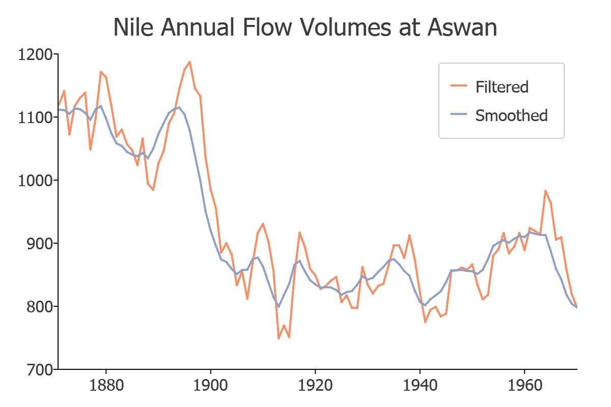
The local level model also produces, via the Kalman filter, an estimate of the unobserved trend component of inflation. When plotted with the observed inflation rate, we can see that the unobserved component appears to be a smoothed version of the observed series.

Once the trend is removed, we are left with the disturbance component. The time series plot of the disturbances suggests that there may still be some regularity in the series that we haven’t accounted for.

Residual Diagnostics
To gain a better idea of the quality of our model, we will run some diagnostic tests on the disturbances.
| Test | Statistic | Probability Value | Conclusion |
|---|---|---|---|
| Ljung-Box test for autocorrelation. | 1.7 | 0.192 | Fail to reject the null hypothesis that the residuals are independently distributed. |
| Test for heteroskedasticity. | 0.289 | 0.000 | Reject the null hypothesis of no heteroskedasticity at the 1% level. |
| Jarque-Bera goodness-of-fit test. | 90.2 | 0.000 | Reject the null hypothesis that the data is normally distributed at the 1% level. |
These results support what we saw in the visualizations of the disturbances - there are remaining patterns in the disturbances that are not accounted for in our model.
Conclusion
Today we've learned more about the simple but powerful local level model. This local level model is a fundamental model that allows us to decompose time series data into unobserved components. This, in turn, helps us better understand the dynamics of our data.

Eric has been working to build, distribute, and strengthen the GAUSS universe since 2012. He is an economist skilled in data analysis and software development. He has earned a B.A. and MSc in economics and engineering and has over 18 years of combined industry and academic experience in data analysis and research.
That;s Great! Could you post the codes? Thanks.
Hello,
This model can be estimated using the GAUSS state space library. The library is in the testing stage but will soon be available for purchase. If you are interested in obtaining the library please email me directly at [email protected]
Eric