Introduction
State-space models provide a powerful environment for modeling dynamic systems. Their flexibility has resulted in a wide variety of applications across fields including radar tracking, 3-D modeling, monetary policy modeling, weather forecasting, and more.
In this blog, we look more closely at state-space modeling using a simple time series model of inflation.
We will cover:
- The components of state-space models.
- Representing state-space models in GAUSS.
- Estimating model parameters using state-space models.
Inflation Modeling
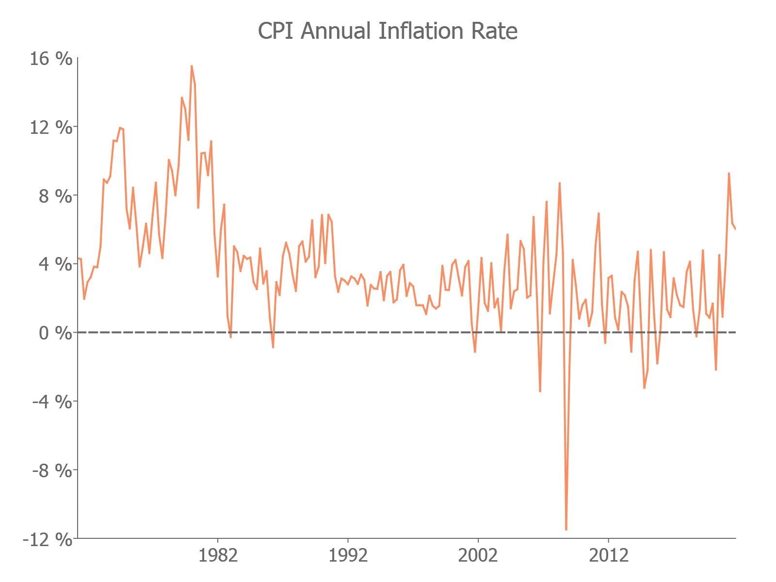
Today we will use the state-space framework to build a simple, albeit naive, model of inflation. This model uses a CPI inflation index, created from the FRED CPIAUCNS average quarterly dataset. Our data ranges from 1971q1 to 2021q4.
State-Space Model Specification
State-space systems specify the dynamics and relationship of two components:
- Observed data.
- Unobserved state variable.
These components are modeled using a measurement equation for the observed data,
$$ y_t = d + Z\alpha_t + \epsilon_t $$
and a transition equation for the unobserved state variable,
$$ \alpha_{t+1} = c + T\alpha_t + R\eta_t $$
where
$$ \epsilon_t \sim N(0, H) $$ $$ \eta_t \sim N(0, Q) $$
and
| Object | Description | Dimension |
|---|---|---|
| $y_t$ | Observed data. | $p \times 1$ |
| $\alpha_t$ | Unobserved data. | $m \times 1$ |
| $d$ | Observation intercept. | $m \times 1$ |
| $Z$ | Design matrix. | $p \times m$ |
| $H$ | Observation disturbance covariance matrix. | $p \times 1$ |
| $c$ | State intercept. | $m \times 1$ |
| $T$ | Transition matrix. | $m \times m$ |
| $R$ | Selection matrix. | $m \times r$ |
| $\eta_t$ | State disturbance. | $r \times 1$ |
| $Q$ | State disturbance covariance matrix. | $r \times r$ |
While this representation may seem simplistic, the framework offers a very flexible platform for modeling. It is used widely in time series analysis including ARIMA, SARIMA, vector autoregressive models, unobserved components, and dynamic factor models.
Example Representation: AR(2) Model
As an example consider an $AR(2)$ model such that
$$ y_t = \phi_1 y_{t-1} + \phi_2 y_{t-2} + e_t $$
$$ e_t \sim N(0, \sigma^2) $$
Let
$$ \alpha_t = (y_t, y_{t-1})' $$
Then we can write our $AR(2)$ model such that
| AR(2) State-space Representation | |
|---|---|
| Measurement Equation | $y_t = \begin{bmatrix} 1 & 0 \end{bmatrix} \alpha_t$ |
| Transition Equation | $\alpha_t = \begin{bmatrix} \phi_1 & \phi_2\\ 1 & 0\end{bmatrix} \alpha_{t-1} + \begin{bmatrix} 1\\ 0 \end{bmatrix} \eta_t$ |
where
| Object | Description |
|---|---|
| $d$ | 0 |
| $Z$ | $\begin{bmatrix} 1 & 0 \end{bmatrix}$ |
| $H$ | 0 |
| $c$ | 0 |
| $T$ | $\begin{bmatrix} \phi_1 & \phi_2\\ 1 & 0 \end{bmatrix}$ |
| $R$ | $\begin{bmatrix} 1 \\ 0 \end{bmatrix}$ |
| $Q$ | $\sigma^2$ |
Example Representation: ARMA(1,1)
The $ARMA(1,1)$ model is given by
$$ y_t = \phi y_{t-1} + \epsilon_t + \theta \epsilon_{t-1} $$ $$ \epsilon_t \sim N(0, \sigma^2) $$
If we let $ \alpha_t = (y_t, \theta \epsilon_t)$ then this can be represented in state-space form such that
| ARMA(1,1) State-space Representation | |
|---|---|
| Measurement Equation | $y_t = \begin{bmatrix} 1 & 0 \end{bmatrix} \alpha_t$ |
| Transition Equation | $\alpha_t = \begin{bmatrix} \phi & 1\\ 0 & 0\end{bmatrix} \alpha_{t-1} + \begin{bmatrix} 1\\ \theta \end{bmatrix} \epsilon_t$ |
where
| Object | Description |
|---|---|
| $d$ | 0 |
| $Z$ | $\begin{bmatrix} 1 & 0 \end{bmatrix}$ |
| $H$ | 0 |
| $c$ | 0 |
| $T$ | $\begin{bmatrix} \phi & 1\\ 0 & 0\end{bmatrix}$ |
| $R$ | $\begin{bmatrix} 1\\ \theta \end{bmatrix}$ |
| $Q$ | $\sigma^2$ |
Estimation of State-Space Models
In most cases, the parameters of our state-space representation are unknown and we wish to estimate them. However, this requires not only estimating the parameters but also estimating the unobserved state variable. Fortunately, we can do both using a combination of the Kalman filter and maximum likelihood estimation.
| Estimating state-space models | |
|---|---|
| Kalman filter | The Kalman filter uses recursive iteration to estimate the unknown state. |
| Maximum likelihood estimation | Uses the likelihood function generated from the Kalman filter to estimate the unknown parameters. |
Let's look at estimating our $ARMA(1,1)$ model using the new sslib library.
The sslib Library
The sslib library is a GAUSS application module for setting up and estimating state-space models.
The state-space library requires:
- A working copy of GAUSS 22+.
- The Constrained Maximum Likelihood MT library for GAUSS.
- The Time Series MT library for GAUSS.
Loading and Transforming Data
To begin our state-space inflation models we need to:
- Load the required libraries:
cmlmt,tsmt, andsslib. - Load the CPI data.
- Calculate the inflation rate.
new;

/*
** Load required libraries
*/
library cmlmt, tsmt, sslib;

/*
** Perform import
*/
cpi_data = loadd(__FILE_DIR $+ "cpi_fred_q_ext.csv", "date($date) + cpi");

// Filter to exclude 2022 data
cpi_data = selif(cpi_data, cpi_data[., "date"] .< "2022");

/*
** Calculate log difference
** annual inflation rate
*/

// Compute log difference rate
y = tsdiff(ln(cpi_data[., "cpi"]), 1);

// Convert from average quarterly decimal
// to annual percentage
y = 4*y*100;

// Rename y variable
y = dfname(y, "Inflation", "cpi");
Setting Up the Parameter Vector and Start Values
Our inflation model has three unknown parameters that we will estimate, $\phi$, $\theta$, and $\sigma^2$. This means our initial parameter vector will be a $3 \times 1$ column vector of starting values.
/*
** Step two: Set up parameter vector
**           and start values
*/
param_vec_st = asDF(zeros(3, 1), "param");

param_vec_st[1] = 0;
param_vec_st[2] = 0;
param_vec_st[3] = 1;Initializing the Control Structure and System Matrices
The sslib uses a ssControl structure to:
- Specify the state-space system matrices.
- Implement stationarity and non-negativity constraints on parameters.
- Control modeling features.
- Specify advanced maximum likelihood controls.
The first step to initializing our model is specifying our model dimensions. These values will be used to initialize the system matrices.
The model dimensions to be specified include:
| Parameter | Description | $ARMA(1,1)$ Model |
|---|---|---|
k_endog | Number of endogenous variables. | 1 |
k_states | Number of state variables. | 2 |
k_posdef | Optional, dimension of the state innovation with positive definite covariance matrix. Default = k_states. | 2 |
/*
** Step three: Set up control structure
**             and model matrices.
*/
// Number of endogenous variables
k_endog = 1;

// Number of states
k_states = 2;
Next we initialize our ssControl structure and set the default system matrices using ssControlCreate:
// Declare and instance of control structure
struct ssControl ssCtl;
ssCtl = ssControlCreate(k_states, k_endog);

// Specify parameter names for output printing
ssCtl.param_names = "phi"$|"theta"$|"sigma2";
Specifying the State-Space Representation
After initializing the state-space system matrices, we are ready to specify our state-space representation. This is done in two separate steps:
- Specify the fixed system matrices that do not contain parameters.
- Specify the matrices which do contain parameters using a custom
updateSSModelfunction.
The system matrices are stored in the initialize ssControl in the ssModel structure named ssm.
| Object | Description | Dimensions |
|---|---|---|
ssm.d | Observation intercept. | $k_{endog} \times k_{states}$ |
ssm.Z | Transition matrix. | $k_{endog} \times 1$ |
ssm.H | Observation disturbance covariance. | $k_{endog} \times k_{endog}$ |
ssm.c | State intercept. | $k_{states} \times 1$ |
ssm.T | Design matrix. | $k_{states} \times k_{states}$ |
ssm.R | Selection matrix. | $k_{states} \times k_{posdef}$ |
ssm.Q | State disturbance covariance. | $k_{states} \times k_{posdef}$ |
ssm.a_0 | Initial prior state mean. | $k_{states} \times 1$ |
ssm.p_0 | Initial prior state covariance. | $k_{states} \times k_{states}$ |
Specifying Fixed System Matrices
To specify the fixed system matrices we use standard matrix assignment:
// Set fixed parameters of model
ssctl.ssm.Z = { 1  0 };
ssctl.ssm.H = 0;
Specifying System Matrices With Parameters
To specify the relationship between the model parameters and the state-space system matrices, we use an updateSSModel procedure. This procedure is then passed to the ssFit procedure for estimation.
The updateSSModel procedure should always contain two inputs:
| Object | Specification |
|---|---|
*ssmod | A pointer to the ssmod structure. |
param | The parameter vector. |
Since this structure uses a pointer to the *ssmod structure, we use the arrow notation, ->, for assigning values to members within the structures.
 /*
** Set up procedure for updating SS model
** structure.
**
*/
proc (0) = updateSSModel(struct ssModel *ssmod, param);

    // Set up kalman filter matrices
    ssmod->R = 1|param[2];
    ssmod->T = (param[1]~1)|(0~0);
    ssmod->Q = param[3];

endp;
Parameter constraints
The final step before estimation is to specify our parameter constraints. For our $ARMA(1,1)$ model we need to:
- Constrain $\phi$ and $\theta$ to be stationary/invertible using the
stationary_varsmember of thessControlstructure. - Constrain $\sigma^2$ to be non-negative using the
positive_varsmember of thessControlstructure.
/*
** Constrained variables
*/

/*
** This stationary_vars member
** indicates which variables should be
** constrained to stationarity.
*/
// Set the first and second parameters in
// the parameter vector to be stationary
ssCtl.stationary_vars = 1|2;

/*
** This positive_vars member
** indicates which variables should be
** constrained to be positive.
*/
// Set the third parameter in
// the parameter vector to be positive
ssCtl.positive_vars = 3;
Estimation
Once the model is specified and the constraints are set, the parameters are estimated using the ssFit procedure. This procedure requires four inputs:
- &updateSSModel
- A pointer to a procedure that updates the state-space system matrices with the parameters.
- param_vec_st
- Vector, starting parameter values.
- y
- Vector, the response data.
- ssCtl
- Structure, an instance of the
ssControlstructure used to control features of the state-space model, Kalman filter, and maximum likelihood estimation.
/*
** Step six: Call the ssFit procedure.
**            This will:
**              1. Estimate model parameters.
**              2. Estimate inference statistics (se, t-stats).
**              3. Perform model residual diagnostics.
**              4. Compute model diagnostics and summary statistics.
*/
struct ssOut sOut;
sOut = ssFit(&updateSSModel, param_vec_st, y, ssCtl);
The ssFit procedure stores results to an ssOut structure and prints estimates, inference statistics, and model diagnostics to screen:
Return Code:                                                             0
Log-likelihood:                                                     -492.4
Number of Cases:                                                       202
AIC:                                                                 990.7
AICC:                                                                990.8
BIC:                                                                  1001
HQIC:                                                                989.7
Covariance Method:                                    ML covariance matrix
==========================================================================

  Parameters   Estimates   Std. Err.      T-stat       Prob.    Gradient
--------------------------------------------------------------------------
         phi      0.9810      0.0160     61.2187      0.0000     -0.0026
       theta     -0.6266      0.0682     -9.1923      0.0000      0.0005
      sigma2      6.5535      0.6537     10.0246      0.0000      0.0000

Wald 95% Confidence Limits
--------------------------------------------------------------------------
  Parameters   Estimates Lower Limit Upper Limit    Gradient
--------------------------------------------------------------------------
         phi      0.9810     -0.8449     -0.6672     -0.0026
       theta     -0.6266      0.5200      1.0881      0.0005
      sigma2      6.5535      2.3061      2.8138      0.0000

Model and residual diagnostics:
==========================================================================

Ljung-Box (Q):                                                        4.12
Prob(Q):                                                            0.0425
Heteroskedasticity (H):                                               1.91
Prob(H):                                                           0.00885
Jarque-Bera (JB):                                                      616
Prob(JB):                                                        1.62e-134
Skew:                                                                 -1.3
Kurtosis:                                                             11.2
==========================================================================
Conclusion
State-space models are powerful and can be used to tackle a wide variety of modeling problems. With a little practice, state-space models can expand your modeling universe substantially.
This blog uses a simple $ARMA(1,1)$ model of inflation to give you a foundation for getting started with state-space models using the GAUSS sslib.
Further Reading
- Filtering Data With the Kalman Filter
- Beginner's Guide to Maximum Likelihood Estimation
- Maximum Likelihood Estimation in GAUSS
- Introduction to the Fundamentals of Time Series Data and Analysis
- Getting Started With Time Series in GAUSS

Eric has been working to build, distribute, and strengthen the GAUSS universe since 2012. He is an economist skilled in data analysis and software development. He has earned a B.A. and MSc in economics and engineering and has over 18 years of combined industry and academic experience in data analysis and research.
Very clear and useful, thanks. I had to change the frequency of the data on FRED to quarterly.
Besides, I changed
to
The code runs smoothly and illustrates very well the theory and the matrixes, and very simple to use.
With my best regards,
Jamel
Hi Jamel,
Thanks for the positive feedback and notes.
Eric
Dear Eric:
I am fresh man for Gauss. If I estimate model about state space , which Librarys are need? I have not purchased none of them, now plan to do it.
Thanks
Dear Eric:
I am sorry, I am freshman. Where is library sslib? I browse the GAUSS Application Modules for paid and github for free library. I can not find it out.
Thank for help.
Hello,
The GAUSS sslib library is in the testing stage but will soon be available for purchase. If you are interested in obtaining the library please email me directly at [email protected]
Eric