The Fundamentals of Kernel Density Estimation

by Eric · Published January 17, 2023

Introduction

In today's blog, we examine a very useful data analytics tool, kernel density estimation. Kernel density estimation (KDE), is used to estimate the probability density of a data sample.

In this blog, we look into the foundation of KDE and demonstrate how to use it with a simple application.

What is Kernel Density Estimation?

Kernel density estimation is a nonparametric model used for estimating probability distributions. Before diving too deeply into kernel density estimation, it is helpful to understand the concept of nonparametric estimation.

Nonparametric Estimation

Unlike traditional estimation techniques, nonparametric estimation does not assume that data is drawn from a known distribution. Rather, nonparametric models determine the model structure from the underlying data.

Examples of Nonparametric Data
Ranked or ordinal data.
Data without a strong theoretical link to a known distribution.
Data with anomalies such as outliers, shifts, or heavy-tails.

Some examples of nonparametric models include:

• Histograms and kernel density estimation.
• Nonparametric regression.
• K-nearest neighbor algorithms.
• Support vector machines.

Probability Distribution Estimation using KDE

The intuition behind KDE is simple -- the more data points in a sample that occur around a location, the higher the likelihood of an observation occurring at that location.

This is implemented by using weighted distances of all observations from various locations on a linearly spaced set of points. Formally, the KDE is given by:

$$\hat{p}_n(x) = \frac{1}{nh} \sum_{i=1}^n K\bigg(\frac{X_i - observation}{h}\bigg)$$

Component	Description
$X_i$	Fixed location.
$K(x)$	The kernel function.
$h$	Smoothing bandwidth.

Don't worry if this equation seems overwhelming. We will look more closely at the components.

The Kernel Function

The kernel function, $K(x)$, specifies how to compute the probability density given the distance, $X_i-observation$. There are a number of kernel functions available and model selection techniques based on mean squared error can be used to help determine which is the best choice for underlying data.

Examples of Kernel Functions
Kernel	Function
Uniform	$k(x) = \frac{1}{2}\\ \text{Support}: |x| \leq 1$
Epanechnikov	$k(x) = \frac{3}{4}(1 - x^2)\\ \text{Support}: |x| \leq 1$
Gaussian	$k(x) = \frac{1}{\sqrt{2\pi}}e^{-\frac{1}{2}x^2}$

Simple Example

Let's consider a simple example:

Observed data	$x_1 = 30, x_2 = 32, x_3 = 35$
Bandwidth ($h$)	5
Linear support	$X_j = \{20, 21, 22, ..., 38, 39, 40\}$
Kernel function	Epanechnikov

Looking at point $x_1 = 30$:

$X_j$	$x_i$	$\frac{X_j - x_i}{h}$	$\frac{3}{4}(1 - x^2)$
20	30	$\frac{20-30}{5} = -1$	$\frac{3}{4}(1 - (-1)^2) = 0$
21	30	$\frac{21-30}{5} = -0.9$	$\frac{3}{4}(1 - (-0.9)^2) = 0.1425$
22	30	$\frac{22-30}{5} = -0.8$	$\frac{3}{4}(1 - (-0.8)^2) = 0.27$
...	...	...	...
38	30	$\frac{38-30}{5} = 0.8$	$\frac{3}{4}(1 - 0.8^2) = 0.27$
39	30	$\frac{39-30}{5} = 0.9$	$\frac{3}{4}(1 - 0.9^2) = 0.1425$
40	30	$\frac{40-30}{5} = 1$	$\frac{3}{4}(1 - 1^2) = 0$

This generates a kernel function centered around the observation $x_1 = 30$:

If we move across all observations we get an individual kernel function for each observation:

To compute the kernel density estimation, we sum the kernel functions at each point.

The Bandwidth

The selected bandwidth controls how smooth the estimated density curve is. There are some convenient things to remember about the bandwidth:

• As we increase bandwidth, points further from our location are included. This results in a smoother distribution.
• Too large of a bandwidth can lead to the loss of information about the shape of the underlying data. This is called oversmoothing.
• Too small of bandwidth may result in the density reflecting randomness rather than our true underlying density. This is called undersmoothing.

Changing the Bandwidth

Now, let's use the previous example to demonstrate the impact of bandwidth selection.

Observations data	$x_1 = 30$
$h$	$h = \{ 5, 10, 15 \}$
Linear support	$X_j = \{20, 21, 22, ..., 38, 39, 40\}$
Kernel function	Epanechnikov

We can see that:

• At the lowest bandwidth, the density goes to zero for $X_j \leq 25$ and $X_j \geq 35$. This results in a steeper and less smooth density.
• The density "widens" as we increase bandwidth, this results in a smoother density.

Empirical Example: Old Faithful

Now let's put our knowledge to use with a real-world example using the Old Faithful dataset, which is available here.

Loading Data

First, we'll load the load data directly from the url:

/*
** Load data from url
*/
url = "https://raw.githubusercontent.com/aptech/gauss_blog/master/econometrics/kernel-density-12-29-22/faithful.csv";
faithful = loadd(url);

The kernelDensity Procedure

Next, we will use the kernelDensity procedure, introduced in GAUSS 23, to estimate the probability density function of the Old Faithful wait times. The kernelDensity procedure requires one input, the data sample.

It also accepts three optional arguments:

• A kernel function specification.
• A bandwidth specification.
• A kernelDensityControl structure for advanced settings.

kd_out = kernelDensity(dataset [, kernel, bw, ctl]);

---

dataset

Name of datafile, dataframe, or data matrix.

kernel

Optional argument, scalar or vector, type of kernel. Default = 1 (Normal).

bw

Optional argument, scalar, vector, or matrix, smoothing coefficient (bandwidth). Must be ExE conformable with the dataset. For example, if scalar, the smoothing coefficient will be the same for each plot. If it is a row vector, there will be a different bandwidth for each column of the dataset. If zero, the optimal smoothing coefficient will be computed. Default = 0.

ctl

Structure, an instance of the kernelDensityControl structure used to control features of estimation including variable names, number of points, truncation, and plot customization.

---

---

Default Estimation

To estimate the kernel density using the default settings and plot the resulting probability density estimate, we can call the kernelDensity procedure with just a single input:

// Estimate and plot the kernel density
call kernelDensity(faithful[., "waittime"]);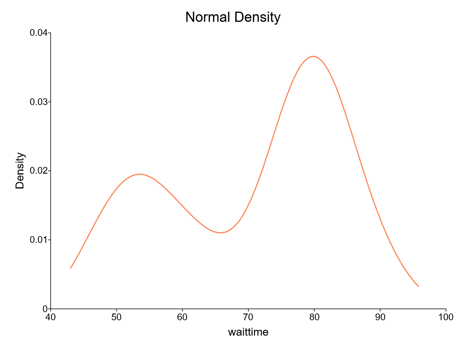

Comparing Kernel Functions

The kernelDensity procedure supports 13 different kernel functions which can be specified using a scalar indicator input:

Supported Kernel Functions
Input	Kernel
1	Normal
2	Epanechnikov
3	Biweight
4	Triangular
5	Rectangular
6	Truncated normal
7	Parzen
8	Cosine
9	Triweight
10	Tricube
11	Logistic
12	Sigmoid
13	Silverman

To compare different kernel functions, we can use a vector input of kernel specifications.

// Specify three kernel
// for comparison on 
// same plot
//   1             Normal
//   3             Biweight
//   5             Rectangular
kernel = { 1, 3, 5}};

// Estimate and plot the kernel density
call kernelDensity(faithful[., "waittime"], kernel);

Changing the Bandwidth

By default GAUSS uses a data-driven rule of thumb to determine the bandwidth. However, the kernelDensity function also accepts a user-specified bandwidth specification. For example, suppose we want to use a bandwidth equal to 2:

// Use the Normal kernel
kernel = 1;

// Set bandwidth 
bw = 2;

// Estimate and plot the kernel density
call kernelDensity(faithful[., "waittime"], kernel, bw);

We can see that this results in a less "smooth" density than our default bandwidth. Conversely, if we use a bandwidth equal to 25:

// Use the Normal kernel
kernel = 1;

// Set bandwidth 
bw = 25;

// Estimate and plot the kernel density
call kernelDensity(faithful[., "waittime"], kernel, bw);

We can see that this results in an oversmoothed density that does not reflect the same data behavior observed with the lower bandwidth.

Conclusion

Today we've looked closely at the fundamentals of kernel density estimation. After reading this blog you should have an understanding of:

• What kernel density estimation is.
• How kernel density estimation works.
• How to perform kernel density estimation in GAUSS.