Introduction
When policy changes or treatments are imposed on people, it is common and reasonable to ask how those people have been impacted. This is a more difficult question than it seems at first glance.
In order to truly know how those individuals have been impacted, we need to consider how those individuals would be had the policies or treatments not taken place. However, the changes did take place, and we don't get to observe how those individuals would fare without those changes.
In today's blog, we examine difference-in-differences (DD) estimation, a common tool for considering the impact of treatments on individuals. We will consider:
- What is difference-in-differences (DD) estimation?
- How does DD work?
- A simple DD example.
What is difference-in-differences estimation

Difference-in-differences estimation attempts to measure the effects of a sudden change in the economic environment, policy, or general treatment on a group of individuals.
The DD model includes several pieces:
- A sudden exogenous source of variation, which we will refer to as the treatment. Treatment examples include changes in minimum wage, a new workplace non-discrimination policy, or a new CO2 emissions tax.
- A quantifiable and measurable outcome which is either the direct target of the variation or an indirect proxy.
- A treatment group which is subjected to the change.
- A control group which is similar in characteristic to the treatment group but is not subjected to the change.
DD uses the outcome of the control group as a proxy for what would have occurred in the treatment group had there been no treatment. The difference in the average post-treatment outcomes between the treatment and control groups is then used to measure the treatment effects.
Example case
Let's consider a simple example. Suppose we have two professors of introductory econometrics classes, one at Transylvania University (TU) and one at The University of Azkaban (UA). Both professors have decided to use GAUSS to teach a year-long series of econometrics courses.
A quarter through the year, the class at TU takes advantage of a free GAUSS training session while the class at UA does not.
We can compare the grades on the GAUSS homework assignments by the students at each university before and after the training date to measure the benefit of the training session.
| Treatment | Aptech GAUSS training course |
|---|---|
| Control Group | Students using GAUSS at University of Azkaban |
| Treatment Group | Students using GAUSS at Transylvania University |
| Outcome | Grades on GAUSS homework assignments |
How does it work?
The DD estimate uses the between-group cross-sectional differences and within-group time-series differences to measure treatment effects. Estimated separately, both the cross-sectional differences and within-group time-series differences may produce biased estimates of the treatment effects.
DD Model Outline
Let's look more formally at our example to better understand how DD works. First, we define our two outcomes
$$Y_{1,i,c,t} = \text{homework grades by student } i \text{, in}\\ \text{ class } c \text{, in period } t \text{ with training course} $$ $$Y_{0,i,c,t} = \text{homework grades by student } i \text{, in}\\ \text{ class } c \text{, in period } t \text{ without training course} $$
where i is an individual student, c is the class and t is the time period.
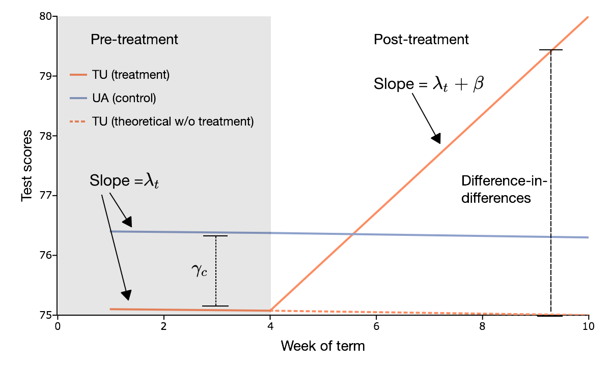
We begin by assuming that potential outcomes before training are determined by a time-invariant, university-specific effect, $\gamma_c$, and a university-invariant, time-specific effect, $\lambda_t$:
$$ E(Y _{0,i,c,t}| c, t) = \gamma_c + \lambda_t $$
Note that the time-invariant component, $\gamma_c$, depends only on the university that the student is in and is independent of the time period. Similarly, the university-invariant component, $\lambda_t$, is independent of the university and changes only with the time period.
Assuming that the training has a constant effect, $\beta$, on homework grades:
$$ E(Y _{1,i,c,t}| c, t) = \gamma_c + \lambda_t + \beta .$$
More generally we can express our outcomes as
$$Y _{i,c,t} = \gamma_c + \lambda_t + \beta D_{c,t} + \epsilon_{i,c,t}$$
where $D_{ct}$ is a dummy variable representing classes that have received training and $E(\epsilon_{ict}| c, t) = 0$.
Using this we compare the differences in outcomes for the individual classes across time:
$$E(Y _{i,c,t} | TU, \text{post-course}) - E(Y _{i,c,t} | TU, \text{pre-course}) =\\ \lambda_{post-course} + \beta - \lambda_{pre-course}$$
and
$$E(Y _{i,c,t} | UA, \text{post-course}) - E(Y _{i,c,t} | UA, \text{pre-course}) =\\ \lambda_{post-course} - \lambda_{pre-course} .$$
From here were are able to estimate the population difference-in-differences which measures the treatment effect of interest
$$ [E(Y _{i,c,t} | TU, \text{post-course}) - E(Y _{i,c,t} | TU, \text{pre-course})] -\\ [E(Y _{i,c,t} | UA, \text{post-course}) - E(Y _{i,c,t} | UA, \text{pre-course})] = \beta .$$
This is the key outcome of the difference-in-differences method. We have eliminated the common trend between the groups, $\lambda_t$, and the permanent differences between the groups, leaving a very simple estimate of the treatment effect, $\beta$.
DD Assumptions
The DD estimation of treatment effects is an appealingly simple way to measure treatment effects. However, it relies on some key assumptions (Angrist and Pischke, 2008):
- Outcomes in the treatment group and the control group follow the same trend, $\lambda_t$.
- The treatment causes deviation, $\beta$, from the trend.
- The differences in the treatment group and control group are captured by the fixed effects variables. $\gamma_c$.
Example
Let's look again at our econometrics students from TU and UA. The students earn the following grades on their assignments:
| Pre-treatment period | Post-treatment period |
|
|---|---|---|
| Transylvania University | 77, 82, 65, 68, 90, 84, 67, 73, 84, 61 | 76, 88, 73, 74, 94, 88, 69, 78, 89, 71 |
| University of Azkaban | 74, 63, 82, 70, 92, 67, 66, 68, 87, 95 | 72, 70, 84, 67, 92, 70, 65, 65, 82, 96 |
Now consider the averages and their differences:
| Pre-treatment period | Post-treatment period | Differences | |
|---|---|---|---|
| Transylvania University | 75.100 (9.235) | 80.000 (8.894) | 4.900 (3.035) |
| University of Azkaban | 76.400 (11.673) | 76.300 (11.383) | -0.100 (3.510) |
| Differences | -1.300 (15.384) | 3.700 (13.166) | 5.000 (3.944) |
The orange highlighted values represent the difference-in-differences across periods between the TU class, the treatment group, and the UA class, the control group. We see that the training class provides a treatment effect of an average 5.00% increase in grades.
The GAUSS code to replicate these results is available on the Aptech GitHub repository.
Conclusion
The difference-in-differences method provides a simple method for estimating treatment effects. The basic two-period approach outlined here provides a foundation for more sophisticated techniques including larger panel regression DD.
In today's blog we have covered the fundamentals of the DD method:
- What is difference-in-differences (DD) estimation
- How does DD work?
- A simple DD example
The code and data for this blog can be found at our Aptech Blog Github code repository.
References
Angrist, Joshua D., and Jörn-Steffen Pischke, 2008, “Mostly harmless econometrics: An empiricist's companion,” Princeton university press.

Eric has been working to build, distribute, and strengthen the GAUSS universe since 2012. He is an economist skilled in data analysis and software development. He has earned a B.A. and MSc in economics and engineering and has over 18 years of combined industry and academic experience in data analysis and research.
These values of std. exist mistakes in typing.
Pingback: Do those not enrolled in Fairtrade arrangements in Malawi still benefit? – Future agricultures
Hallo Eric. I do not understand the meaning of the numbers in parentheses in the table. Can you please explain what they are? Thank you.
Hello Massimo,
Thank you for your question. The number in the parentheses is the standard error of the means.
Eric