Example overview
Autoregressive models take the general form:
$$ y_t = x_t \beta_t + u_t\\ u_t - \phi_1 u_{t-1} - \ldots - \phi_p u_{t-p} = e_t\\ e_t \sim N(\theta, \sigma^2) $$
The time series module provides a number of routines for performing pre-estimation data analysis, model parameter estimation, and post-estimation diagnosis of autoregressive time series.
Preliminary and Partial Autocorrelations
Suppose we have stationary univariate time series data but are uncertain about the order of the regressive relationship. You may wish to first use the sample autocorrelation function to help identify the general structure of the model. This can be achieved in GAUSS using the autocormt and autocovmt functions.
autocormt
The autocormt function computes the autocorrelations for each column of a matrix. It assumes that all data has been demeaned and produces an output matrix containing the autocorrelations for each column of an input matrix.
autocormt requires three input arguments:
- X
- An N x K data matrix.
- f
- A scalar denoting the first autocorrelation to be computed
- l
- A scalar denoting the last autocorrelation to be computed.
Consider a time series that follows the purely autoregressive data generation process given by:
$$ y_t = 1.5 + u_t\\ u_t - 0.5u_{t-1} + 0.8u_{t-2} = e_t\\ e_t \sim N(0,1) $$
Realizations of any ARMA data generation process can be randomly created using the function simarmamt:
// Load TSMT library
library tsmt;

// Specify ARMA Parameters
b_sim =  { 0.5, -0.8 };

// Specify MA order
q_sim = 0;

// Specify AR order
p_sim = 2;

// Specify deterministic features (constant and trend)
const_sim = 1.5;
tr_sim = 0;

// Number of observations
n_sim = 200;

// Number of series to simulate
k_sim = 4;

// Standard deviation of the error terms
std_sim = 1;

// Set seed for repeatable simulations
seed_sim = 5012;

// Perform simulation
y_sim = simarmamt(b_sim,p_sim,q_sim,const_sim,tr_sim,n_sim,k_sim,std_sim,seed_sim);

/*
** Visualize data
*/
x_plot = seqa(1,1,rows(y_sim));

// Draw graph
plotXY(x_plot, y_sim[.,1]);
The code above will produce a 200X4 matrix of data that follows the AR(2) data generating process specified. Each column of the matrix represents a different random realization of the process. The code graphs the first realization (the first column of y_sim):

Though the data generating process of the data above is known, it is generally more realistic that one will wish to estimate the parameters of an unknown data generating process behind a realization of data. To begin, consider finding the ACF and the PACF using the GAUSS autocor and pacf functions:
/*
** Find autocorrelations for 0 to 10 lags
*/

// Create 'y' by demeaning each column of 'y_sim'
y = y_sim - meanc(y_sim)';

// Find autocorrelations
first = 0;
last = 10;
a = autocor(y_sim, first, last);

// Display autocorrelations
a_lab = seqa(0,1,rows(a));
print "Lags"$~"ACF";
print ntos(a_lab~a, 4);
This code calculates and lists the sample autocorrelations for lags 0 through 10 for each sample of data. All columns of the list have a precision of two decimal points. Column labels “Lags” and “ACF” are included at the top of the list. This list will change depending on the data that has been randomly generated but should look similar to:
Lags           ACF
   0             1             1             1             1
   1         0.511         0.589         0.598         0.556
   2        -0.158        0.0363        0.0987        0.0105
   3       -0.0824        0.0527         0.152         0.135
   4         0.524         0.501         0.571         0.588
   5         0.745         0.751         0.741         0.685
   6         0.343         0.545         0.497         0.373
   7       -0.0297         0.223         0.229         0.175
   8         0.139         0.171         0.276         0.363
   9          0.53          0.39         0.485         0.552
  10         0.559         0.579         0.587         0.456
As an alternative, a bar graph visually presents the autocorrelation information. For example,
/*
** Display Correlogram
*/

// Declare 'myPlot' to be a plotControl structure
// and fill with default values for bar plots
struct plotControl myPlot;
myPlot = plotGetDefaults("bar");

// Add a title
plotSetTitle(&myPlot, "Correlogram");

// Add axes labels
plotSetYLabel(&myPlot, "ACF");
plotSetXLabel(&myPlot, "Lag");

// Draw graph
x_lag = seqa(0, 1, 11);
plotBar(myPlot, x_lag, a[1:rows(a),1]);
This produces the following output:

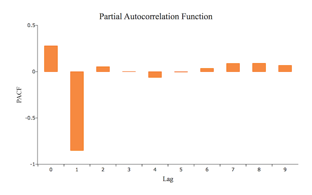
The pacf function supplements the diagnostic information in the ACF and finds the partial autocorrelation function. The previous example is easily extended to find the PACF for the same randomly generated data. The pacf function requires three inputs:
- x
- An N x 1 data vector.
- k
- A scalar denoting the maximum number of partial autocorrelation to compute.
- d
- A scalar denoting the order of differencing.
Note that in GAUSS the pacf function always begins with the minimum of one lag. Hence, if k=10, pacf will find the partial autocorrelations for lags 1 through 10. For example,
// Find PACF
b = pacf(y[1:rows(y),1], 10, 0);

// Display partial autocorrelations
b_lab = seqa(0, 1, rows(b));
print "";
print "Lags"$~"PACF";
print ntos(b_lab~b, 2);

/*
** Plot PACF
*/

// Declare 'myPlot' to be a plotControl structure
// and fill with default values for bar plots
struct plotControl myPlot;
myPlot = plotGetDefaults("bar");

// Add a title
plotSetTitle(&myPlot, "Partial Autocorrelation Function");

// Add axis labels
plotSetYLabel(&myPlot, "PACF");
plotSetXLabel(&myPlot, "Lag");

// Plot PACF
plotBar(myPlot, b_lab,b);
This code calculates, lists, and graphs the partial autocorrelations for lags 0 through 10. This list and graph will change depending on the data that has been randomly generated but should look similar to:
Lags        PACF

    0       0.28
    1      -0.85
    2      0.054
    3     0.0018
    4     -0.062
    5     -0.004
    6      0.035
    7      0.089
    8      0.091
    9      0.068
Estimating the Autoregressive Model
The arimamt function is a convenient tool for estimating the parameters of any ARIMA model, including ARMA models, purely AR models, and purely MA models. The arimamt function takes two arguments:
- ctl
- An
arimamtcontrol structure. - y
- N x 1 data vector
Note that this function can only be used to estimate models with a specified number of sequentially ordered lags. For example, it will estimate the parameters for the first through fourth lag but will not estimate a model that includes ONLY the first and fourth lag. In addition, note that this arimamt will produce an error if the data is not stationary and invertible.
The arimamt Control Structure
This structure handles the matrices and strings that control the estimation process such as specifying whether to include a constant, output appearance and estimation parameters.
Continuing with the example above,
// Declare 'ctl' to be an arimamtControl structure
// and fill with default values
struct arimamtControl ctl;
ctl = arimamtControlCreate();

// Declare 'out' to be an arimamtOut structure,
// to hold the results from 'arimamt'
struct arimamtOut out;

// Specify the AR order to 2
ctl.ar = 2;

// Specify order of differencing
ctl.diff = 0;

// Specify MA order
ctl.ma = 0;

// Include constant in model (default)
ctl.const = 1;
This appropriately passes to arimamt that the model is an AR(2) model and includes a constant. The remaining control elements (the ones that we did not set above), left at the default values, specify preferences for output display and estimation.
With the control structure options set, we can now perform the estimation:
// Perform estimation with 'arimamt'
out = arimamt(ctl, y_sim[.,1]);
which will return output similar to:
Model:  ARIMA(2,0,0)

Final Results:

Log Likelihood:    718.584998         Number of Residuals: 200

AIC           :  -1433.169996         Error Variance     : 1.056229913

SBC           :  -1426.573361         Standard Error     : 1.027730467


DF: 198      SSE: 209.133522700


 Coefficients     Std. Err.   T-Ratio    Approx. Prob.
AR[1,1] 0.51943    0.03673    14.14024   0.00000

AR[2,1]-0.85411    0.03654   -23.37306   0.00000


Constant:   1.89661768
Total Computation Time: 0.13 (seconds)

AR Roots and Moduli:

Real :    0.30407   0.30407
Imag.:    1.03843  -1.03843
Mod. :    1.08204   1.08204
Forecasting
We will produce forecasts from our model, using tsforecastmt. It takes five inputs:
- ctl
- An arimamtControl structure which, as we saw above, contains the AR and MA order of the model.
- b
- A vector of parameter estimates, possibly returned by
arimamt. - y
- A time series vector from which to produce forecasts.
- e
- A vector of errors, possibly returned from
arimamt. - h
- A scalar, the number of periods to forecast.
tsforecastmt returns a matrix with three columns, containing the lower forecast bound, the forecast and the upper forecast bound. Continuing on with our example, we will produce a 10 period forecast:
//Produce 10 period forecast
f = tsforecastmt(amc, amo.b, y_sim[.,1], amo.e, 10);
will return output similar to:
Forecasts for ARIMA(2,0,0) Model.   95% Confidence Interval Computed.

 Period        LCL        Forecasts        UCL     Forecast Std. Err.
   201      0.104811      2.124232      4.143652      1.030336
   202     -0.461607      1.813988      4.089582      1.161039
   203     -0.904040      1.659289      4.222618      1.307845
   204     -1.130503      1.843919      4.818340      1.517590
   205     -0.910903      2.071950      5.054802      1.521891
   206     -1.264531      2.032700      5.329932      1.682292
   207     -1.523356      1.817549      5.158454      1.704575
   208     -1.726063      1.739318      5.204698      1.768084
   209     -1.707635      1.882446      5.472526      1.831707
   210     -1.578898      2.023608      5.626114      1.838047
The Command File
Finally we put it all together in the command file below, which will reproduce all output shown above.
// Load TSMT library
library tsmt;

/*
** Step 1: Simulate
*/

// Specify ARMA Parameters
b_sim =  { 0.5, -0.8 };

// Specify MA order
q_sim = 0;

// Specify AR order
p_sim = 2;

// Specify deterministic features (constant and trend)
const_sim = 1.5;
tr_sim = 0;

// Number of observations
n_sim = 200;

// Number of series to simulate
k_sim = 4;

// Standard deviation of the error terms
std_sim=1;

// Set seed for repeatable simulations
seed_sim = 5012;

// Perform simulation
y_sim = simarmamt(b_sim,p_sim,q_sim,const_sim,tr_sim,n_sim,k_sim,std_sim,seed_sim);

// Visualize data
obs_num = seqa(1,1,rows(y_sim));

// Declare 'myPlot' to be a plotControl structure
// and fill with default values for xy plots
struct plotControl myPlot;
myPlot = plotGetDefaults("xy");

// Add a title
plotSetTitle(&myPlot, "AR(2) Data Simulation", "Times", 18);

// Set X and Y Axis labels
plotSetXLabel(&myPlot, "Observation");
plotSetYLabel(&myPlot, "Y");

// Plot 'y' observations
plotXY(myPlot, obs_num, y_sim[.,1]);

/*
** Step 2: ACF and PACF
*/

// Create 'y' by demeaning each column of 'y_sim'
y = y_sim - meanc(y_sim)';

// Find autocorrelations
first = 0;
last = 10;
a = autocor(y_sim, first, last);

// Display autocorrelations
a_lab = seqa(0,1,rows(a));
print "Lags"$~"ACF";
print ntos(a_lab~a, 4);

// Fill 'myPlot' with default values for bar plots
myPlot = plotGetDefaults("bar");

// Open new graphics tab so that we do not
// draw over our previous graph
plotOpenWindow();

// Add a title
plotSetTitle(&myPlot, "Correlogram", "Times", 18);

// Add axes labels
plotSetYLabel(&myPlot, "ACF");
plotSetXLabel(&myPlot, "Lag");

// Plot ACF
x_lag = seqa(0, 1, 11);
plotBar(myPlot, x_lag, a[1:rows(a),1]);

// Find PACF
b = pacf(y[1:rows(y),1], 10, 0);

// Display partial autocorrelations
b_lab = seqa(0, 1, rows(b));
print "";
print "Lags"$~"PACF";
print ntos(b_lab~b, 2);

// Add a title
plotSetTitle(&myPlot, "Partial Autocorrelation Function");

// Add axis labels
plotSetYLabel(&myPlot, "PACF");
plotSetXLabel(&myPlot, "Lag");

// Open new graphics tab so that we do not
// draw over our previous graph
plotOpenWindow();

// Plot PACF
plotBar(myPlot, b_lab,b);

/*
** Step 3: Estimate
*/

// Declare 'amc' to be an arimamtControl structure
// and fill with default values
struct arimamtControl amc;
amc = arimamtControlCreate();

// Declare 'amo' to be an arimamtOut structure,
// to hold the results from 'arimamt'
struct arimamtOut amo;

// Specify the AR order to 2
amc.ar = 2;

// Specify order of differencing
amc.diff = 0;

// Specify MA order
amc.ma = 0;

// Include constant in model (default)
amc.const = 1;

// Perform estimation with 'arimamt'
amo = arimamt(amc, y_sim[.,1]);

/*
** Step 4: Forecast
*/

/ /Produce 10 period forecast
f = tsforecastmt(amc, amo.b, y_sim[.,1], amo.e, 10);