TSMT 2.1: Rolling and Recursive OLS Estimation

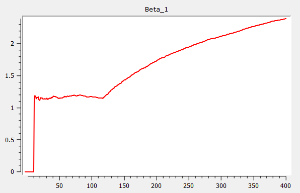
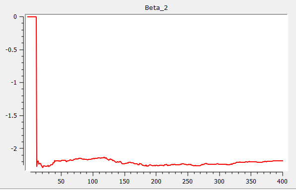
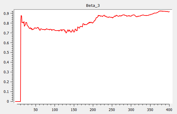
Example: Rolling estimation procedure

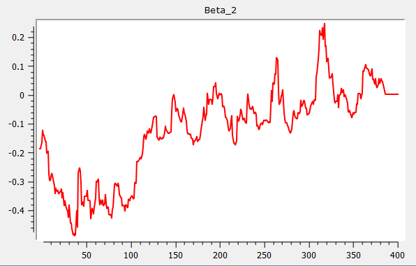
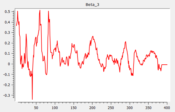
This example uses 400 observations of generated data with a break in the intercept after 120 observations. The error terms are standard normal. The data is replicated using the code below:

//Load TSMT library
library tsmt;
 
//Parameters for before (b1) and after (b2) break
b1 = { 1.2, -2, 0.75 };
b2 = { 5, -2, 0.75 };
 
//Number of observations before break
n1 = 120;
 
//Total number of observations
n_tot = 400;
 
//Simulate observations and error term
xt = ones(n_tot,1)~rndn(n_tot,2);
err = rndn(n_tot,1);
 
//Create series with break
y1 = xt[1:n1,.]*b1 + err[1:n1,.];
y2 = xt[n1+1:n_tot,.]*b2 + err[n1+1:n_tot,.];
yt_break = y1|y2;

Next we set the parameters to run a rolling window regression on the data simulated above and run the regression.

//Set-up expanding window size
wind = 15;
 
//Add specifies increment to increase window size by
//and is irrelevant for rolling window regression
add = 15;
 
//Gr is an indicator for graphing
gr = 1;
 
{ beta, res, w } = rolling(yt_break, xt, wind, add, gr);

Which produces the following three graphs for Beta 1, Beta 2 and Beta 3:

Finally we set parameters to run a forward expanding window regression and run the regression.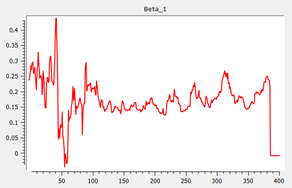

//Set-up expanding window size
wind = -15;
 
//Add specifies increment to increase window size by
//and is irrelevant for rolling window regression
add = 15;
 
//Gr is an indicator for graphing
gr = 1;
 
{ beta_fwd, res_fwd, w_fwd } = rolling(yt_break, xt, wind, add, gr);

Which produces the following three graphs for Beta 1, Beta 2 and Beta 3:

‹ ›