
Goals
This tutorial builds on the previous Linear Regression and Generating Residuals tutorials. It is suggested that you complete those tutorials prior to starting this one.
This tutorial demonstrates how to test the OLS assumption of homoscedasticity. After completing this tutorial, you should be able to :
- Plot the squared residuals against predicted y-values.
- Run the Breusch-Pagan test for linear heteroscedasticity.
- Perform White's IM test for heteroscedasticity.
Introduction
In this tutorial, we examine the residuals for heteroscedasticity. If the OLS model is well-fitted there should be no observable pattern in the residuals. The residuals should show no perceivable relationship to the fitted values, the independent variables, or each other. A visual examination of the residuals plotted against the fitted values is a good starting point for testing for homoscedasticity. However, it should be accompanied by statistical tests.
Plot residuals versus fitted values
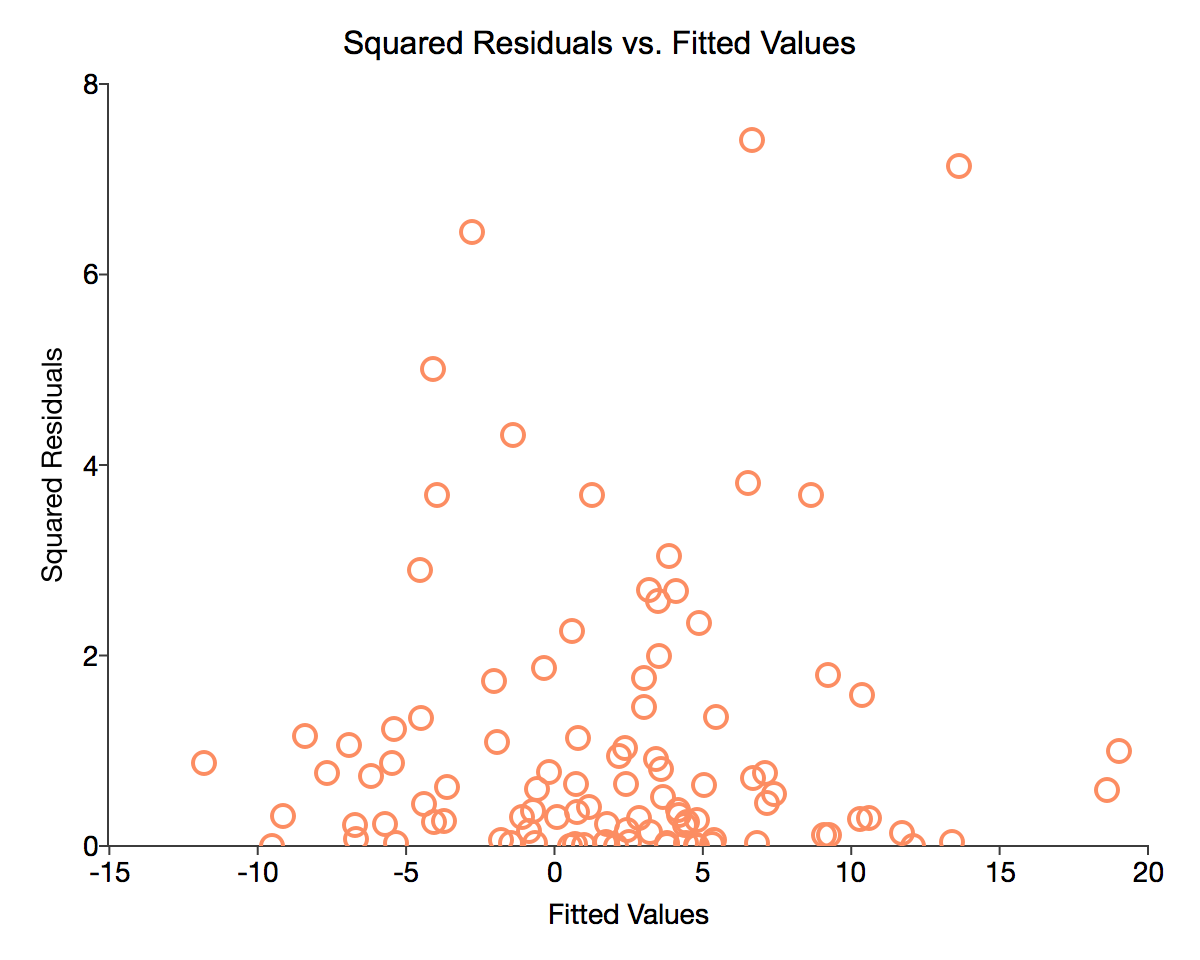
Our first diagnostic test will be to visually examine a chart of the residuals versus predicted y-values. As demonstrated in the previous tutorial, we have stored the residuals computed by the ols function in the variable resid. Using these residuals we compute the predicted y
$$\hat{Y} = X\hat{\beta}$$
// Add ones to x for constant
x_full = ones(num_obs, 1)~x;

// Predicted y values
y_hat = x_full*b;
Charting the residuals versus the fitted y values allows us to look for any visual patterns of relationships between the fitted values and the error terms.
/*
** Plot histogram of residuals
** Set format of graph
** Declare plotControl structure
*/
struct plotControl myPlot;

// Fill 'myPlot' with default scatter settings
myplot = plotGetDefaults("scatter");

// Add title to graph
plotSetTitle(&myPlot, "Squared Residuals vs. Fitted Values", "Arial", 16);
plotSetXLabel(&myPlot, "Fitted Values");
plotSetYLabel(&myPlot, "Squared Residuals");

// Create scatter plot
plotScatter(myPlot, y_hat, resid.*resid);
The code above should produce a graph similar to the image below:
Breusch-Pagan Test
The Breusch-Pagan test for heteroscedasticity is built on the augmented regression
$$ \frac{\hat{e}_i^2}{\hat{s}_i^2}\ = \alpha + z_it + \nu_i $$
where $ e_i $ is a predicted error term resid, $ s_i^2 $ is the estimated residual variance and $ z_i $ can be any group of independent variables, though we will use the predicted y values from our original regression. To conduct the Breusch-Pagan tests we will:
- Square and rescale the residuals from our initial regression.
- Regress the rescaled, squared residuals against the predicted y values from our original regression.
- Compute the test statistic.
- Find the critical values from the chi-squared distribution with one degree of freedom.
1. Square and rescale the residual from the original regression
Before running the test regression we must construct the dependent variable by rescaling the squared residuals from our original regression. The rescaling is done by dividing the squared residual by the average of the squared residuals. The result, a variable with a mean of 1, will become the dependent variable in our test regression.
/*
** Square the residuals
** The .* operator provides element-by-element multiplication
*/
sq_resid = resid .* resid;

// Find average of squared residuals
average_ssr = meanc(sq_resid);

// Rescale squared error
rescaled_sq_resid = sq_resid / average_ssr;
2. Run the augmented regression
In order to construct the test statistic, we must run the augmented regression
$$\frac{\hat{e}_i^2}{\hat{s}_i^2}\ = \alpha + z_it + \nu_i $$
where $ e_i $ is a predicted error term, $ s_i^2 $ is the estimated residual variance and $ z_i $ can be any group of independent variables, though we will use the predicted y values from our original regression.
// Dependent variable in augmented regression
bp_y = rescaled_sq_resid;

// Independent variable in augmented regression
bp_z = y_hat;

// Run ols
{ bp_nam, bp_m, bp_b, bp_stb, bp_vc, bp_std,
  bp_sig, bp_cx, bp_rsq, bp_resid, bp_dbw } = ols("", bp_y, bp_z);
The code above should produce the following output report:
Valid cases:                100      Dependent variable:                   Y
Missing cases:                0      Deletion method:                   None
Total SS:               197.036      Degrees of freedom:                  98
R-squared:                0.003      Rbar-squared:                    -0.008
Residual SS:            196.508      Std error of est:                 1.416
F(1,98):                  0.263      Probability of F:                 0.609
Durbin-Watson:            2.149

                        Standard                Prob   Standardized  Cor with
Variable     Estimate     Error      t-value    >|t|     Estimate    Dep Var
-----------------------------------------------------------------------------
CONSTANT     0.97528   0.149584    6.519966     0.000       ---         ---
X1           0.01250   0.024379    6.519966     0.609    0.051733    0.051733
3. Construct test statistic
The Breusch-Pagan test statistic is equal to the augmented model sum of squares divided by two.
// Find predicted y
bp_y_hat = x_full*bp_b;

// Find regression sum of squares
bp_tmp = (bp_y_hat - meanc(bp_y));
bp_rss = bp_tmp'*bp_tmp;
4. Find the test statistic critical values
The Breusch-Pagan statistic is distributed Chi-square (1). In general, high values of the test statistic imply homoscedasticity and indicate that the ols standard errors are potentially biased. Conversely, low values provide support for the alternative hypothesis of heteroscedasticity. More specifically, we should use the built in GAUSS function cdfChic can be used to find the p-value of the test statistic. cdfChic takes the following inputs:
- x
- Matrix, abscissae values for chi-squared distribution
- n
- Matrix, degrees of freedom.
// Calculate test statistic
bp_test = bp_rss/2;
print "Chi Square(1) =" bp_test;

// Calculate p-value
prob = cdfChic(bp_test, cols(y_hat));
print "Prob > chi2 = " prob;
The above code should print the following output:
Chi Square(1) =   0.034952371
Prob > chi2 =     0.85169550
Our chi-square test statistic is very small and the p-value for our test statistic is 85.2%, exceeding 5%. This indicates that we cannot reject the null hypothesis of homoscedasticity.
White's IM Test
White's IM test offers an alternative test for homoscedasticity based on the r-squared from the augmented regression
$$ e_i^2 = \alpha + x_1 + x_2 + ... + x_i + x_1^2 + x_2^2 + ... +x_i^2 + x_1x_2 + x_2x_3 + ... + x_ix_j + \nu_i $$
The test statistic of $ N * R^2 $ tests the null hypothesis of homoscedasticity and has a chi-square distribution with $ \frac{K*(K+3)}{2}\ $ degrees of freedom.
1. Construct matrix of independent variables
Since we created the squared residuals for the previous test, we just need to construct the RHS variables for our augmented regression. In this case, we have only one independent variable in our original regression and our augmented regression equation is
$$ e_i^2 = \alpha + x_1 + x_1^2 + \nu_i $$
/*
** Construct independent variables matrix
** The tilde operator '~' provides horizontal
** concatenation of matrices
*/
im_z = x ~ x.^2;
2. Run the augmented regression
We can use our newly created matrix im_z
// Dependent variable in augmented regression
im_y = sq_resid;

// Run ols
{ im_nam, im_m, im_b, im_stb, im_vc, im_std,
  im_sig, im_cx, im_rsq, im_resid, im_dbw } = ols("",im_y,im_z);
The above code will print the following report:
Valid cases:                100      Dependent variable:                   Y
Missing cases:                0      Deletion method:                   None
Total SS:               226.453      Degrees of freedom:                  97
R-squared:                0.003      Rbar-squared:                    -0.018
Residual SS:            225.807      Std error of est:                 1.526
F(2,97):                  0.139      Probability of F:                 0.871
Durbin-Watson:            2.148

                        Standard                Prob   Standardized  Cor with
Variable     Estimate     Error     t-value     >|t|     Estimate    Dep Var
-----------------------------------------------------------------------------
CONSTANT     1.05013    0.18120    5.79548     0.000       ---         ---
X1           0.07032    0.15796    0.44520     0.657    0.047440    0.051733
X2           0.01277    0.09751    0.13093     0.896    0.013951    0.028548
3. Construct test statistic
The final step is to find the test statistics $ N*R^2 $. This statistic is distributed Chi-square with $ \frac{K*(K+3)}{2}\ $ degrees of freedom. We again use the function cdfChic to find the p-value of the test statistic.
// Calculate test statistic
im_test = num_obs*im_rsq;
print "IM test" im_test;

// Find degrees of freedom
K = (cols(im_z));
im_dof = (K*(K+3))/2;
print "Degrees of freedom:" im_dof;

// Calculate p-value
prob = cdfChic(im_test, im_dof);
print "Prob > chi2 = " prob;
The above code should print the following output:
IM test      0.28524914
Degrees of freedom:       5.0000000
Prob > chi2 =       0.99791134
The White IM test is consistent with the findings from our Breusch-Pagan test. Our chi-square test statistic is again very small and the p-value is greater than 5%. This means we cannot reject the null hypothesis of homoscedasticity.
Conclusion
Congratulations! You have:
- Plotted the squared residuals against predicted y-values.
- Computed the Breusch-Pagan test for linear heteroscedasticity.
- Computed White's IM test for heteroscedasticity.
The next tutorial examines methods for testing for influential data.
For convenience, the full program text is below.
// Clear the work space
new;

// Set seed to replicate results
rndseed 23423;

// Number of observations
num_obs = 100;

// Generate independent variables
x = rndn(num_obs, 1);

// Generate error terms
error_term = rndn(num_obs,1);

// Generate y from x and errorTerm
y = 1.3 + 5.7*x + error_term;

// Turn on residuals computation
_olsres = 1;

// Estimate model and store results in variables
screen off;
{ nam, m, b, stb, vc, std, sig, cx, rsq, resid, dbw } = ols("", y, x);
screen on;

print "Parameter Estimates:";
print b';

/**************************************************************************************************/
// Add ones to x for constant
x_full = ones(num_obs, 1)~x;

// Predicted y values
y_hat = x_full*b;

/*
** Plot histogram of residuals
** Set format of graph
** Declare plotControl structure
*/
struct plotControl myPlot;

// Fill 'myPlot' with default scatter settings
myplot = plotGetDefaults("scatter");

// Add title to graph
plotSetTitle(&myPlot, "Squared Residuals vs. Fitted Values", "Arial", 16);
plotSetXLabel(&myPlot, "Fitted Values");
plotSetYLabel(&myPlot, "Squared Residuals");

// Create scatter plot
plotScatter(myPlot, y_hat, resid.*resid);
/**************************************************************************************************/
/*
** Square the residuals
** The .* operator provides element-by-element multiplication
*/
sq_resid = resid .* resid;

// Find average of squared residuals
average_ssr = meanc(resid'*resid);

// Rescale squared error
rescaled_sq_resid = sq_resid / average_ssr;

// Dependent variable in augmented regression
bp_y = rescaled_sq_resid;

// Independent variable in augmented regression
bp_z = y_hat;

// Run ols
{ bp_nam, bp_m, bp_b, bp_stb, bp_vc, bp_std,
  bp_sig, bp_cx, bp_rsq, bp_resid, bp_dbw } = ols("", bp_y, bp_z);

// Find predicted y
bp_y_hat = x_full*bp_b;

// Find regression sum of squares
bp_tmp = (bp_y_hat - meanc(bp_y));
bp_rss = bp_tmp'*bp_tmp;

// Calculate test statistic
bp_test = bp_rss/2;
print "Chi Square(1) =" bp_test;

// Calculate p-value
prob = cdfChic(bp_test, cols(y_hat));
print "Prob > chi2 = " prob;
/**************************************************************************************************/
/*
** Construct independent variables matrix
** The tilde operator '~' provides horizontal
** concatenation of matrices
*/
im_z = x ~ x.^2;

// Dependent variable in augmented regression
im_y = sq_resid;

// Run ols
{ im_nam, im_m, im_b, im_stb, im_vc, im_std,
  im_sig, im_cx, im_rsq, im_resid, im_dbw } = ols("", im_y, im_z);

// Calculate test statistic
im_test = num_obs*im_rsq;
print "IM test" im_test;

// Find degrees of freedom
K = (cols(im_z));
im_dof = (K*(K+3))/2;
print "Degrees of freedom:" im_dof;

// Calculate p-value
prob = cdfChic(im_test, im_dof);
print "Prob > chi2 = " prob;