
Example: VAR Model in TSMT
Vector autoregressive models generalize the single variable autoregressive model to allow for more than one endogenous variable. The standard (or reduced) form of a VAR(1) model with two separate time series is:
yt,1 = α1 + φ11 yt-1,1 +φ1,2 yt-1,2 + ut,1
yt,2 = α2 + φ21 yt-1,1 +φ22 yt-1,2 + ut,2
Assuming:
- y is an N by p matrix, where N is the length of the time series and p is the order of the VAR.
- alpha is a 1 by p matrix, representing the intercept term.
- e is an N by p matrix containing the error term.
We can express a VAR(p) model in matrix form, using GAUSS code as:
y[t,1:p] = alpha + y[t-1,.] * phi' + e[t,.];Load and plot time series
For this example, we will use a data set that comes with TSMT, named minkmt.asc. This file contains data for the prices of two commodities from 1850 to 1910. The first column contains the dates and the second and third columns contain the data.
//Get path to GAUSSHOME directory
path = getGAUSSHome();

//Add file name to path
fname = path $+ "examples/minkmt.asc";

//Load data from the second and third columns
//of a space separated text file
y = csvReadM(fname, 1, 2|3, " ");

//Load first date
first_date = csvReadM(fname, 1|1, 1|1, " ");

//Plot data
plotTS(first_date, 1, y);
The above code should produce a plot that looks similar to this:
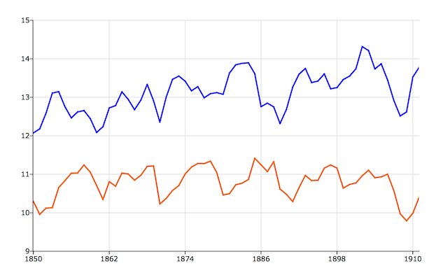
The first thing that we notice is that the, at least the first series, seems to have a trend and that neither series has a mean near zero. We can use the TSMT function, vmdetrendmt to remove the trend and demean the data. The vmdetrendmt function takes two inputs:
- An NxK matrix containing one or more time series to be acted upon.
- A scalar, indicator variable with the following options:
0 Return the original data untouched. 1 Detrend the data, based upon a linear model. 2+ Detrend the data based upon a polynomial model.
Now we will detrend and demean our data, assuming only a linear trend.
//Load TSMT library functions
library tsmt;

//Detrend and demean data
y_detrend = vmdetrendmt(y, 1);

//Plot transformed data
plotTS(first_date, 1, y_detrend);
The graph of the detrended data should look more like this:
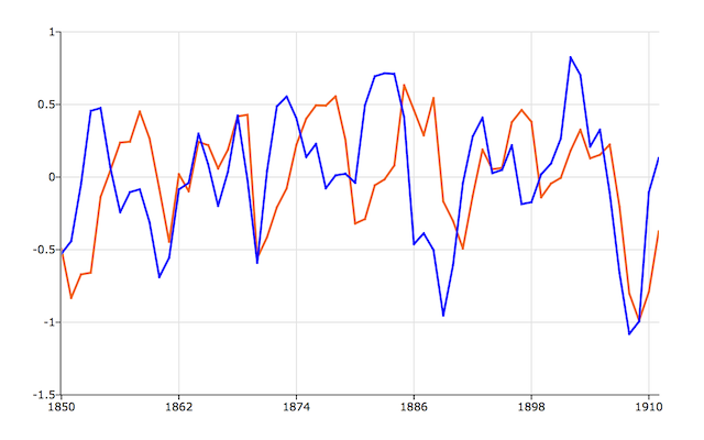
After detrending, the data appears to have a mean of zero and does not have a trend. However, the variance of the data seems to increase with time. Let's try differencing the data instead of detrending:
//Calculate the first difference
y_diff = vmdiffmt(y, 1);

//Plot transformed data
plotTS(first_date, 1, y_diff);
The plot of the differenced data should look like this:
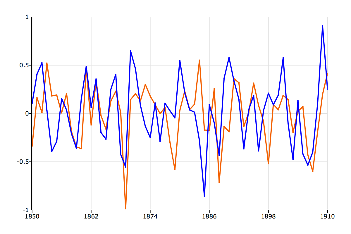
This plot does not appear to have a trend, the mean is near zero and the variance does not appear to increase with time.
Estimating the Vector Autoregressive Model
The varmaxmt function is a convenient tool for estimating the parameters of VAR models with or without exogenous variables. The varmaxmt function takes two required arguments:- A varmamtControl structure.
- An N x K data vector, y, where each column of y is a different time series.
The varmamtControl Structure
This structure handles the matrices and strings that control the estimation process such as specifying whether to include a constant, output appearance, and estimation parameters. Continuing with the example above,//Declare 'vctl' to be a varmamtControl structure
//and fill with default values
struct varmamtControl vctl;
vctl = varmamtControlCreate();
//Declare 'vout' to be an varmamtOut structure,
//to hold the results from 'varmaxmt'
struct varmamtOut vout;
//Specify the AR order to 2
vctl.ar = 2;
//Specify order of differencing
vctl.diff = 1;
//Specify MA order
vctl.ma = 0;
//No constant in model
vctl.const = 0;//Perform estimation with 'varmaxmt'
//Note that we are passing in the original, 'y'
//Since we told 'varmaxmt' to difference 'y',
//by setting vctl.diff = 1
vout = varmaxmt(vctl, y);===============================================
VARMAX Version 2.1.3
===============================================
Phi
Plane [1,.,.]
-0.12309 0.57672
-0.67611 0.34425
Plane [2,.,.]
0.26190 -0.12894
-0.26000 -0.044378
standard errors
Plane [1,.,.]
1.0000 1.0000
1.0000 1.0000
Plane [2,.,.]
1.0000 1.0000
1.0000 1.0000
t-values
Plane [1,.,.]
-0.12309 0.57672
-0.67611 0.34425
Plane [2,.,.]
0.26190 -0.12894
-0.26000 -0.044378
probabilities
Plane [1,.,.]
0.90253 0.56672
0.50209 0.73210
Plane [2,.,.]
0.79447 0.89792
0.79593 0.96478
Residual Covariance Matrix
0.066376 0.026428
0.026428 0.065819
standard errors
1.0000 1.0000
1.0000 1.0000
t-values
0.066376 0.026428
0.026428 0.065819
probabilities
0.94734 0.97902
0.97902 0.94778
Beta0
-0.010973
0.021210
Augmented Dickey-Fuller UNIT ROOT Test for Y1
Critical Values
ADF Stat 1% 5% 10% 90% 95% 99%
No Intercept -5.2278 -2.5328 -1.9498 -1.6266 0.9152 1.3168 2.1179
Intercept -5.1774 -3.5663 -2.9370 -2.6152 -0.4393 -0.0499 0.6942
Intercept and Time Trend -5.2981 -4.0892 -3.4615 -3.1709 -1.2584 -0.9195 -0.2986
Augmented Dickey-Fuller UNIT ROOT Test for Y2
Critical Values
ADF Stat 1% 5% 10% 90% 95% 99%
No Intercept -4.7720 -2.5328 -1.9498 -1.6266 0.9152 1.3168 2.1179
Intercept -4.7352 -3.5663 -2.9370 -2.6152 -0.4393 -0.0499 0.6942
Intercept and Time Trend -4.6155 -4.0892 -3.4615 -3.1709 -1.2584 -0.9195 -0.2986
Phillips-Perron UNIT ROOT Test for Y1
PPt 1% 5%
No Intercept -7.2621 -2.5328 -1.9498
Intercept -6.9186 -3.5663 -2.9370
Intercept and Time Trend -6.9497 -4.0892 -3.4615
Phillips-Perron UNIT ROOT Test for Y2
PPt 1% 5%
No Intercept -6.3499 -2.5328 -1.9498
Intercept -5.9127 -3.5663 -2.9370
Intercept and Time Trend -5.8505 -4.0892 -3.4615
Augmented Dickey-Fuller COINTEGRATION Test for Y1 Y2
Critical Values
ADF Stat 1% 5% 10% 90% 95% 99%
No Intercept -5.0448 -3.4003 -2.8198 -2.4901 -0.2841 0.1628 0.9912
Intercept -5.0375 -4.0246 -3.4040 -3.0890 -0.9988 -0.6383 0.0929
Intercept and Time Trend -5.1691 -4.5041 -3.9157 -3.6062 -1.6464 -1.3413 -0.6750
Johansen's Trace and Maximum Eigenvalue Statistics. r = # of CI Equations
Critical Values
r Trace Max. Eig 1% 5% 10% 90%
No Intercept 0 65.5906 46.3981
1 19.1925 19.1925 1.0524 1.7046 2.1927 9.3918
Intercept 0 65.6102 46.4140
1 19.1962 19.1962 2.2515 3.3599 4.0975 12.8635
Intercept and Time Trend 0 66.2392 46.3986
1 19.8406 19.8406 4.0389 5.3796 6.1879 16.1762
Dep. Variable(s) : Y1 Y2
No. of Observations : 61 61
Degrees of Freedom : 50 50
Mean of Y : 0.0018 0.0279
Std. Dev. of Y : 0.3014 0.3506
Y Sum of Squares : 5.4509 7.3772
SSE : 4.0489 4.0150
MSE : 0.0730 0.0723
sqrt(MSE) : 0.2701 0.2690
R-Squared : 0.2572 0.4558
Adjusted R-Squared : 0.1086 0.3469
Model Selection (Information) Criteria
......................................
Likelihood Function : -2.0830
Akaike AIC : -17.8339
Schwarz BIC : 49.3857
Likelihood Ratio : 4.1661
Characteristic Equation(s) for Stationarity and Invertibility
AR Roots and Moduli:
Real : 4.2121928 -1.9895302
Imag.: 0.0000000 0.0000000
Mod. : 4.2121928 1.9895302
MULTIVARIATE ACF
LAG01 LAG02 LAG03
0.03143 0.06429 -0.1224 -0.0856 -0.0715 -0.1648
0.002152 -0.03561 -0.1163 -0.2181 0.133 0.1341
LAG04 LAG05 LAG06
-0.1864 -0.1613 -0.1483 0.09278 -0.3151 0.02871
-0.04398 -0.04798 0.01561 -0.04506 -0.1768 -0.03803
LAG07 LAG08 LAG09
0.008986 -0.02272 -0.04262 0.01081 0.2493 0.3194
-0.04619 -0.1493 -0.09121 0.06298 0.1083 0.08513
LAG10 LAG11 LAG12
0.4103 0.04377 0.01628 -0.1909 -0.01679 0.005056
0.1636 -0.1654 0.1557 0.1854 -0.09051 0.07984
ACF INDICATORS: SIGNIFICANCE = 0.95
(using Bartlett's large sample standard errors)
LAG01 LAG02 LAG03 LAG04 LAG05 LAG06
-+-+ -+-+ -+-+ -+-+ -+-+ -+-+
-+-+ -+-+ -+-+ -+-+ -+-+ -+-+
LAG07 LAG08 LAG09 LAG10 LAG11 LAG12
-+-+ -+-+ -+-+ -+-+ -+-+ -+-+
-+-+ -+-+ -+-+ -+-+ -+-+ -+-+
Multivariate Goodness of Fit Test
Lag Qs P-Value
3 9.5468 0.0488
4 12.4737 0.1313
5 17.3960 0.1353
6 26.3349 0.0495
7 28.0138 0.1091
8 29.4429 0.2039
9 38.2221 0.0943
10 55.2182 0.0066
11 64.9744 0.0022
12 66.9787 0.0048Forecasting
We will produce forecasts from our model, using vmforecastmt. It takes five inputs:
- A varmamtControl structure which, as we saw above, contains the AR order and other model settings.
- A varmamtOut structure, possibly returned by varmaxmt, which will contain the parameter estimates for our VAR model.
- A time series vector from which to produce forecasts. The length of this vector must be (p + 1), where p is the specified order of the AR process. However, vmforecast will read from the end of the vector. This allows you to pass in the entire time series if you want forecasts from the end of your data.
- A vector or matrix, containing any exogenous variables in the model over the forecast horizon.
- A scalar, the number of periods to forecast.
vmforecastmt returns a matrix in which the first column contains the forecast observation number (from 1 to the number of forecast periods), the remaining columns contain the forecast for each of the endogenous variables. Continuing on with our example, we will produce a 10 period forecast:
//Produce 10 period forecast
//Since we have no exogenous variables,
//we pass a scalar zero for the 4th input
f = vmforecastmt(vctl, vout, y, 0, 10);
The forecast matrix, f should look similar to this:
1 0.437 0.222
2 0.0291 -0.286
3 0.151 -0.338
4 -0.0829 -0.242
5 -0.169 -0.213
6 -0.0461 -0.0513
7 -0.0927 0.0731
8 -0.0407 0.0669
9 0.0481 0.102
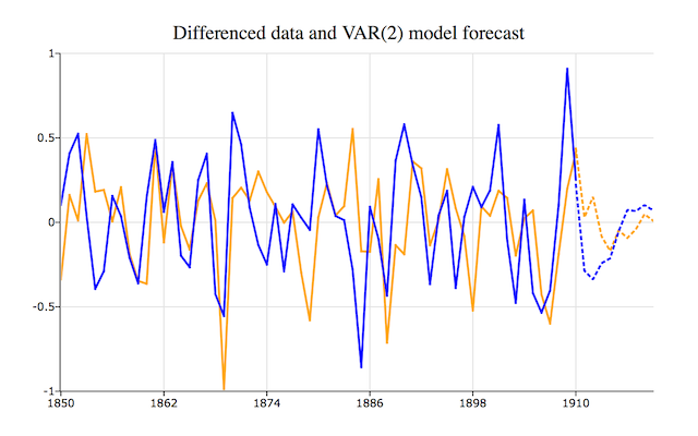
10 0.00988 0.0714After calculating our forecast, we can plot the original differenced data and our forecasts together like this:
//Declare 'myPlot' to be a plotControl structure
struct plotControl myPlot;

//Fill 'myPlot' with default values
myPlot = plotGetDefaults("xy");

//Set line colors
plotSetLineColor(&myPlot, "orange"$|"blue");

plotSetTitle(&myPlot, "Differenced data and VAR(2) model forecast", "times", 18);

//Plot differenced 'y' data
plotTS(myPlot, 1850, 1, y);

//Set line style dots for forecast period
plotSetLineStyle(&myPlot, 3);

//Add forecasts to plot
plotAddTS(myPlot, 1910, 1, f[.,2:3]);
Which should produce the following graph.
The Command File
Finally we put it all together in the command file below, which will reproduce all output shown above.//Load TSMT library functions
library tsmt;
/*******************************************
** **
** Load and process data **
** **
*******************************************/
//Create file name with full path
fname = getGAUSSHome() $+ "examples/minkmt.asc";
//Load all rows of the second and third columns of
//a space separated file
y = csvReadM(fname, 1, 2, " ");
//Difference the data
y = vmdiffmt(y, 1);
/*******************************************
** **
** Estimate **
** **
*******************************************/
//Declare 'vctl' to be a varmamtControl structure
struct varmamtControl vctl;
//Fill 'vctl' with default values
vctl = varmamtControlCreate();
//Specify a VAR(2) model
vctl.ar = 2;
//Declare 'vout' to be a varmamtOut structure
//to hold the return values from 'vout'
struct varmamtOut vout;
//Estimate the parameters of the VAR(2) model
//and print diagnostic information
vout = varmaxmt(vctl, y);
/*******************************************
** **
** Forecast **
** **
*******************************************/
//Create a 10 period forecast
f = vmforecastmt(vctl, vout, y, 0, 10);
/*******************************************
** **
** Plot differenced data and forecast **
** **
*******************************************/
//Declare 'myPlot' to be a plotControl structure
struct plotControl myPlot;
//Fill 'myPlot' with default values
myPlot = plotGetDefaults("xy");
//Set line colors
plotSetLineColor(&myPlot, "orange"$|"blue");
plotSetTitle(&myPlot, "Differenced data and VAR(2) model forecast", "times", 18);
//Plot differenced 'y' data
plotTS(myPlot, 1850, 1, y);
plotSetLineStyle(&myPlot, 3);
//Add forecasts to plot
plotAddTS(myPlot, 1910, 1, f[.,2:3]);